Analysis of Activity Pattern of Children Attending Elementary School, and Development of a Prediction Model Based on Data Mining Approach for ADHD Screening

저작자표시-비영리-동일조건변경허락 2.0 대한민국 이용자는 아래의 조건을 따르는 경우에 한하여 자유롭게 l 이 저작물을 복제, 배포, 전송, 전시, 공연 및 방송할 수 있습니다. l 이차적 저작물을 작성할 수 있습니다. 다음과 같은 조건을 따라야 합니다: l 귀하는, 이 저작물의 재이용이나 배포의 경우, 이 저작물에 적용된 이용허락조건 을 명확하게 나타내어야 합니다. l 저작권자로부터 별도의 허가를 받으면 이러한 조건들은 적용되지 않습니다. 저작권법에 따른 이용자의 권리는 위의 내용에 의하여 영향을 받지 않습니다. 이것은 이용허락규약(Legal Code)을 이해하기 쉽게 요약한 것입니다. Disclaimer 저작자표시. 귀하는 원저작자를 표시하여야 합니다. 비영리. 귀하는 이 저작물을 영리 목적으로 이용할 수 없습니다. 동일조건변경허락. 귀하가 이 저작물을 개작, 변형 또는 가공했을 경우 에는, 이 저작물과 동일한 이용허락조건하에서만 배포할 수 있습니다.

Analysis of Activity Pattern

of Children Attending Elementary School,

and Development of a Prediction Model Based on

Data Mining Approach for ADHD Screening

by

Hye Jin Kam

Major in Medicine

Department of Medical Sciences

The Graduate School, Ajou University

Analysis of Activity Pattern

of Children Attending Elementary School,

and Development of a Prediction Model Based on

Data Mining Approach for ADHD Screening

by

Hye Jin Kam

A Dissertation Submitted to The Graduate School of Ajou University

in Partial Fulfillment of the Requirements for the Degree of

Ph. D. in Medical Sciences

Supervised by

Rae Woong Park, M.D., Ph.D.

Major in Medicine

Department of Medical Sciences

The Graduate School, Ajou University

This certifies that the dissertation

of Hye Jin Kam is approved.

SUPERVISORY COMMITTEE

Jai Sung Noh

Rae Woong Park

KiYoung Lee

Ki Woong Kim

Peom Park

The Graduate School, Ajou University

December 23rd, 2010

i - ACKNOWLEDGEMENT - 돌아보면, 다사다난했던 박사학위과정 3 년 반의 시간 중 기억하지 못하는 때가 대부분이지만, 처음 학교를 향하는 버스에서 설레임과 기대감은 지금도 또렷하게 기억합니다. 그 때의 저로부터 지금의 저는 얼마나 달라져 있을까요? 제 자신은 그 때와 별반 다를 것이 없는 것 같은데, 어느 새 저를 둘러싸고 있는 세상이 달라져 있다는 생각이 듭니다. 어쩌면, 짧지만은 않았던 그 시간 동안 여러 사건과 사람들을 만나고 지나오면서 세상만이 아니라 제 자신도, 모르는 사이 조금은 자라고 더 깊이 뿌리를 내리게 되었는지도 모르겠습니다. 이제 조그만 언덕 위에 올라서며 둘러보니, 제가 지나온 오솔길도 보이고 앞서거니 뒤서거니 하며 언덕으로 오르고 있는 사람들도 보입니다. 산들바람이 불어오는 뒤편으로는 이곳을 지나간 많은 사람들이 저 높은 산을 향해 걸어가고 있는 모습들도 눈에 들어오네요. 구름에 가려 그 높이와 형태도 미처 그려낼 수 없는 그런 산입니다. 그 산에는 무엇이 있을까요? 꼭대기를 향한 길에서는 무엇이 또 누가 저를 기다리고 있을까요? 굳이 저 산을 오르지는 않아도 될 겁니다. 하지만, 또 다른 어떤 길을 선택하더라도 어느 즈음엔 또 다른 산을 만나게 되겠지요. 그리고, 산을 오르는 것이 힘들지 만은 않을 거라는 믿음이 있습니다. 걸어가는 길목 길목에서 달콤한 샘과 시원한 바람, 그리고 즐거운 사람들도 만날 수 있을 겁니다. 이미 이곳을 향하면서 경험했던 것처럼 말이지요. 제가 어림짐작으로 상상하는 그 산의 꼭대기와 그곳을 향하는 길이 어쩌면 엉터리인지도 제가 그 끝에 이를 수 있을지도 모를 일입니다. 하지만 그것이 산으로 향하는 발걸음을 잡지는 않길 바랍니다. 제 목표는 산 꼭대기가 아니라 포기하지 않고 산을 오르는 것에 있으니까요.

ii 제가 지금 여기 이 언덕까지 이르기까지의 동안에도 크고 작은 사건들이 있었겠지요. 기억에도 떠오르지 않는 소소한 일상의 사건들부터 지금 떠올려도 커다란 파도같이 부딪쳐오는 일들도 있었네요. 그리고 많은 사람들이 있었습니다. 의료 정보학이라는 새로운 학문의 길을 보여주신 박래웅 교수님, 이곳에서 다시 뵙게 된 생활 연구인 이기영 교수님, 듬직한 랩장이자 애처가인 사랑이 아빠 우재, 손이 많이 가긴 하지만 정 많은 또 다른 애처가 동기 만영, 늘 사람 사는 얘기가 가득해서 왠지 하루가 24 시간 이상일 것 같은 연구 파트너 은경, 같은 고향이라는 이유로 억울(?)하게 제 라인이라는 오해를 받기도 했던 멀티 테스킹의 지존 덕용, 연구실의 크고 작은 일들이 원만하게 흘러갈 수 있게 많은 도움을 주는 동시에 심신이 건강한 바른 생활을 해야 한다는 압박을 주는 혜경 선생님, 쉴 틈 없이 바쁘신 중에도 학업에 대한 열의를 불태우시는 입학 동기 백설경 팀장님, 심신이 바쁜 워킹맘이면서도 멋지게 석사학위를 쟁취(?)해 낸 성진옥 선생님, 그리고 선배로 후배로 동료로 친구로 연구과제로 업무로 만났던 좋은 사람들의 얼굴이 떠오릅니다. 그리고, 언덕을 오르는 동안 기쁘고 신났던 순간들 힘들고 아팠던 시간 모두를 함께 했고 앞으로도 함께 해 줄 사랑하는 가족들이 있습니다. 멀리서도 응원과 믿음을 보내주셨던 사랑하는 아빠와 엄마, 떠올리기만 해도 든든한 오빠, 늘 아껴주시고 응원과 칭찬을 아끼지 않으셨던 시댁 가족들, 그리고 언제 어떻게 무엇을 하던지 무엇이 되어있던지 늘 빛처럼 그림자처럼 함께 해주는 남편에게 깊은 믿음과 신뢰를 마음으로부터 보냅니다. 모두들 고맙습니다. 2010 년 12 월 감 혜 진 드림

iii - ABSTRACT -

Analysis of Activity Pattern of Children Attending Elementary

School, and Development of a Prediction Model

Based on Data Mining Approach for ADHD Screening

Questionnaire-based attention deficit disorder with hyperactivity (ADHD) screening tests may not always be objective or accurate, owing to both subjectivity and prejudice. Despite attempts to develop objective measures to characterize ADHD, no widely applicable index currently exists. The principal aim of this study was to determine whether high-resolution activity features could provide a sufficient analytical foundation for determining the activity transitions of children with ADHD and to develop a decision support model for ADHD screening by monitoring children’s school activities using a 3-axial actigraph. Actigraphs were placed on the non-dominant wrists of 153 children for 3 hours, while they were at school. Children who scored high on the questionnaires were clinically examined by child psychiatrists, who then confirmed ADHD. Mean, variance, and ratios of activity within partitioned activity regions (a unit of 0.1G) were extracted as activity features. As a primary research on the effect by contexts of school life, activity features were extracted for three courses, including art, language and math. And, they were compared between the ADHD and non-ADHD groups via principal component analysis (PCA) and other statistical analyses. For, screening model construction, two decision tree models were constructed using the C5.0 algorithm after feature selection step: [A] from

iv

whole hours (class + playtime) and [B] during classes. Accuracy, sensitivity, and specificity were evaluated. Positive/negative predictive value, odds ratio, relative risk, likelihood ratio and area under ROC curve (AUC) were also calculated for model evaluation.

In the comparison analysis on course contents, especially in the art course, the two groups of children were almost completely separable by the new features, and the activity distributions of the groups differed significantly over a broad range. Those findings also showed that the course contents appeared to influence the activity patterns of children with ADHD. Monitoring the actual magnitude and counts of activity over a broad range could facilitate deeper investigations into the distributions or patterns of activities. And, two 5-depth decision trees were constructed by C5.0 algorithms. [Model A] three non-ADHD children were misclassified, resulting in an accuracy score of 97.89%. Sensitivity and NPV were 1.00. Specificity and PPV were 0.98 and 0.58-0.77, respectively. [Model B] 11 non-ADHD children were misclassified, resulting in an accuracy score of 92.23%. Specificity and PPV were scored at 0.92 and 0.27-0.47, respectively. Objective screening of latent ADHD patients can be accomplished with a simple watch-like sensor, which is worn for just a few hours while the child attends school. The model proposed herein can be applied to a great many children without heavy cost in time and manpower cost, and would generate valuable results from a public health perspective.

Key words: Attention deficit disorder with hyperactivity, Classroom behavior, Activity monitoring, Activity level, Activities of daily living, Actigraph, Decision support

v

TABLE OF CONTENTS

ACKNOWLEDGEMENT ··· i

ABSTRACT ··· iii

TABLE OF CONTENTS ··· iv

LIST OF FIGURES ··· vii

LIST OF TABLES ··· ix

I. INTRODUCTION A. BACKGROUNDS ··· 1

B. STUDY AIMS ··· 8

II. MATERIALS AND METHODS A. STUDY OVERVIEW ··· 9

B. PARTICIPANTS ··· 11

1. RECRUITMENTS & QUESTIONNAIRES ADMINISTRATION ··· 11

2. PARTICIPANTS SELECTION WITH CLINICAL DIAGNOSIS ··· 12

C. ELEMENTARY SCHOOL IN KOREA ··· 14

D. ACTIVITY MEASUREMENT & INFORMATION ACUISITION ··· 15

E. COMPARISONS OF SITUATIONAL EFFECT ON ACTIVITY PATTERNS 17 1. OVERVIEW ··· 17

2. FEATURE EXTRACTION ··· 19

3. PINCIPAL COMPONENT ANALYSIS (PCA) ··· 23

vi

F. MODEL CONSTRUCTION FOR ADHD SCREENING ··· 26

1. OVERVIEW OF MODEL CONSTRUCTION ··· 26

2. FEATURE EXTRACTION & SELECTION ··· 28

3. DECISION TREE MODEL CONSTRUCTION ··· 32

4. SOLVING CLASS IMBALANCE PROBLEM ··· 36

5. MODEL EVALUATION & STATISTICAL ANALYSIS ··· 38

III. RESULTS A. COMPARISONS OF ACTIVITY PATTERNS ··· 44

1. PARTICIPANT SELECTION ··· 44

2. PCA ANALYSIS ··· 46

3. STATISTICAL ANALYSIS ··· 48

B. SCREENING MODEL CONSTRUCTION ··· 65

1. PARTICIPANT SELECTION ··· 65

2. SELECTE ACTIVITY FEATURES ··· 67

3. CONSTRUCTED SCREENING MODELS ··· 69

4. COMPARISON WITH SELECTED FEATURES ··· 73

5. MODEL EVALUATION ··· 75

IV. DISCUSSION A. COMPARISONS OF SITUATIONAL EFFECT ON ACTIVITY PATTERNS 1. ACTIVITY DISTRIBUTION ··· 78

2. THE EFFECTS OF SITUATIONAL DEMANDS INVOLVING RESCTRICTIONS ··· 80

vii

B. MODEL CONSTRUCTION FOR ADHD SCREENING ··· 82

1. SCREENING MODELS FOR ADHD BY MONITORING CHILDREN’S ACTIVITY ··· 82

2. SIGNIFICANCE OF SELECTED FEATURES ··· 86

3. APPLICABILITY ··· 88

C. LIMITATIONS ··· 90

V. CONCLUSION ··· 93

REFERENCES ··· 95

viii

LIST OF FIGURES

Fig. 1. Study overview: Analysis of activity pattern of children attending elementary

school, and development of a screening model for ADHD ··· 10

Fig. 2. A picture of the actigraphs that were used for the activity data acquisition ··· 15

Fig. 3. Overview of the study on situational effects on the activity of children with and without ADHD at school ··· 18

Fig. 4. Sample data of 3-axial activities corded into ADHD data mart ··· 19

Fig. 5. Comparisons between two sample children’s vector summed activity values ··· 20

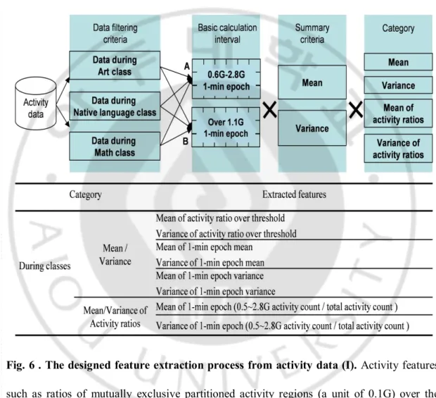
Fig. 6. The designed feature extraction process from activity data (I) ··· 21

Fig. 7. Overview of the process-flow for ADHD screening model construction: (A) a general process for screening & diagnosis of ADHD and (B) process to build screening models for ADHD with activity features ··· 27

Fig. 8. The designed feature extraction process from activity data (II) ··· 29

Fig. 9. An example of the receiver operating characteristic curve (ROC curve) ··· 43

Fig. 10. Three-dimensional views of activity characteristics of children with and without ADHD using the features extracted based on proposed ‘actigraph’ ··· 47

Fig. 11. Distribution of activity features for ADHD and non-ADHD groups according to each course ··· 49

Fig. 12. Activity distribution graphs of ADHD and non-ADHD group between courses ··· 58

ix

Fig. 13. Constructed decision trees for screening ADHD: (A) Model A (whole hours) and (B) Model B (class hours) ··· 70 Fig. 14. The distributions of scores were compared between well-classified and

x

LIST OF TABLES

Table 1. A general type of confusion matrix for prediction results ··· 38

Table 2. Results of systematic questionnaire and clinical confirmation ··· 44

Table 3. Demographic and clinical characteristics of children with and without ADHD ··· 45

Table 4. Between group analysis: standard error (SE), p-values (p) and effect size (ES) ··· 53

Table 5. Within group analysis for children with ADHD: standard error (SE), p-values (p) and effect size (ES) ··· 59

Table 6. Within group analysis for children without ADHD: standard error (SE), p-values (p) and effect size (ES) ··· 62

Table 7. Demographic and clinical characteristics of children with and without ADHD ··· ··· 66

Table 8. Selected activity features ··· 68

Table 9. Selected input features for tree construction ··· 72

Table 10. Comparison of activity levels with regard to selected features ··· 74

- 1 -

I. INTRODUCTION

A. Backgrounds

Attention-deficit hyperactivity disorder (ADHD) is one of the most common childhood neurobehavioral disorders, and has been estimated to affect 3-9% of school-age children (Goodyear & Hynd, 1992; Kofler et al., 2008; Teicher et al., 1996). ADHD is characterized by difficulties with attention, impulse control, and hyperactivity relative to typical children of the same age and gender; it has also been shown to lead to impairments in several important domains of functioning. Children with ADHD commonly experience difficulties in completing their schoolwork and also tend to under-achieve academically (Morein-Zamir et

al., 2008). ADHD has been implicated in up to 10-fold increases in the incidence of

antisocial personality disorder, and up to 5-fold increases in the risk of drug abuse (Teicher

et al., 1996). Therefore, early diagnosis and treatment are necessary for children who suffer

from ADHD.

It is commonly agreed that children with ADHD tend to be more hyperactive than children without ADHD (Halperin et al., 1993; Porrino et al., 1983). Some past studies of activity level in children with ADHD have reported that their excessive movement was ubiquitous rather than situation specific (Porrino et al., 1983), whereas other seminal studies and recent experimental studies have demonstrated that activity levels are situation-specific (Antrop et al., 2005; Purper-Ouakil et al., 2004; Whalen et al., 1978). Clinicians must carefully record psychomotor-activity levels and their clinical impressions of patients.

- 2 -

Regardless of the skill of the clinician, however, the signs of ADHD are notoriously variable and situational in nature. A single assessment over a brief visit may not be reflective of the patient’s general level of activity or impairment (Teicher, 1995). Consequently, clinicians frequently rely heavily on impressions and scorings from schoolteachers or parents, which are neither consistently objective nor accurate (Teicher, 1996). However, the signs of ADHD vary in different situations, and assessments based on short-period activity may not reveal the key characteristic of ADHD (Teicher, 1995). Fluctuations in the symptoms of ADHD may complicate its diagnosis. Considering that unfamiliar environments or situations may mitigate or aggravate the symptoms of ADHD, it is important to consider environmental contexts in the observational research and diagnosis of children with ADHD.

Beyond teacher reports, direct observation of students in their classroom, as compared to laboratory or clinical interviews, is an important means of understanding the characteristics of ADHD (Lauth et al., 2006). It has been previously noted that a classroom situation with a high stimulation level (noise, visual distracters and a large class size) was likely to elicit the primary characteristics of ADHD. Moreover, detailed knowledge regarding the classroom behavior of children with ADHD is necessary to establish many of the criteria required for a diagnosis, and proper management and teaching depend on thorough knowledge of the in-class behavior of such children (Lauth et al., 2006). Several studies have been previously conducted to monitor the activities of children with ADHD in naturalistic classroom environments. For example, Antrop et al. (2005) performed a comparison study to confirm the effects of the combination of time of day and playtime

- 3 -

using situational variables including the degree of out-of-seat behavior, non-productive repetitive movements and inattention to class activities or off-task behavior. They reported that minordifferential effects of time of day and playtime exerted minor differential effects

on the hyperactive behavior of children with ADHD as comparedto that of control children,

specifically with regard to noisiness and out-of-_{seat behavior (Antrop et al., 2005). Lauth et} al. (2006), in another example, monitored the classroom activities of children with ADHD

via external observers. The children with ADHD’s off-task and on-task behavior (such as regular lesson with interaction, regular lesson with minimal interaction, and non-instructional context) were compared, and showed that children with ADHD were more disruptive and inattentive than their counterparts.

In this study, actigraphs were applied in an effort to non-invasive observe long-term changes in children’s activity (Swanson et al., 2002). Activity is a complicated data situation, which reflects continuous and multi-dimensional changes in body position (Laerhoven et al., 2006). An actigraph is an electronic device which can simplify and quantify complex activity information into numerical values; this process involves activity recognition and classification, both subjects that are studied extensively in the artificial intelligence and pervasive computing communities (Pärkkä et al., 2006; Choudhury et al., 2006; Hong et al., 2005; Liao et al., 2005). Actigraphs have also been used in several studies to evaluate alterations in body position that precede falls in elderly individuals (Burchfield et al., 2007; Zhang et al., 2005; Chen et al., 2005). The actigraph, in this case, helped to overcome the conditional limits inherent to such an effort, and allowed for long-term monitoring of

- 4 -

patients’ activity. Posture and motion patterns, according to many researchers and theorists, are key indicators of emotional state (Laerhoven et al., 2006). An actigraph, then, can also be used to record motor activity in individuals suffering from psychiatric disorders; this approach has already been applied to the analysis and study of individuals with Parkinson’s disease and akathisia (Tuisku et al., 2003; Tuisku et al., 1994; van Someren et al., 2006). The most profound merit of the actigraph is that it allows for a patient’s activity information to be obtained in a natural setting for a prolonged and continuous period (Teicher, 1995; Tuisku et al., 1999; Tuisku et al., 2003; van Someren et al., 2006).

Several methods for the objective measurement of the activity levels of children with ADHD were previously developed using actigraphs (Gruber et al., 2006; Halperin et al., 1992; Halperin et al., 1993; Porrino et al., 1983; Tsujii et al., 2007). Children suffering from ADHD tend to be more active, restless, and fidgety than typical children. A number of previous studies have been conducted to develop objective measures, define hyperactivity, and quantify disturbances in attention or impulse, as compared to children without ADHD, by employing the behavioral characteristics evidenced by children with ADHD. Hyperactivity is one of the diagnostic criteria of ADHD. Activity scores were compared with the scores of continuous performance tests (CPT) with activity (Halperin et al., 1992): activity was measured with wrist-worn activity sensors during assessment sessions of the ADHD and control children, and the correlations of the CPT scores and activity features from the actigraph were evaluated. The results of these evaluations demonstrated significant differences in activity levels between the ADHD and non-ADHD. Many actigraphy studies

- 5 -

have corroborated this significant difference in activity between children with and without ADHD. Children with ADHD have been shown to be 20-30% more active than children without ADHD in school- or laboratory-based attention tasks, as determined by analyzing data generated by wearable actigraphs (Porrino et al., 1983; Halperin et al., 1992). Tsujii et

al. (2007) attempted to determine whether any association could be drawn between activity

level and situational factors (Tsujii et al., 2007). They compared the mean activity of children with ADHD and controls in morning and afternoon classes, by dividing class hours into four cases: in-seat, not in-seat, physical education, and lunch/recess time. In their study, ADHD patients and controls wore actigraphs for 1 week while attending an elementary school, and the maximum difference in activity level between the two groups was noted when the effects of inhibition and fatigue overlapped ADHD. They reported a sizeable difference in the mean activity between the two groups during the afternoon in-seat class period. In another study, differences in the activity levels of the two groups were noted (average and standard deviation) during recess time; however, no difference between the groups was detected during the in-seat class period (Tsujii et al., 2009).

These previous studies, however, utilized only limited activity information, such as means of or variances in the entire activity. Preexisting accelerometers were used to actigraphically assess subjects’ activities over the long term, by generating counts or summaries of activity in excess of a pre-defined temporal threshold: these measures did not designate the actual ‘amount’ or degree of activity, but rather the mere ‘frequency’ of intervals in which high levels of activity above a certain pre-defined threshold, and thus It

- 6 -

have hypothesized that they could not provide the series of informative features necessary to determine distribution or patterns of a wide range of activities. These long-term measurements rendered it possible to evaluate subjects’ activity levels quantitatively; however, this approach is also limited in that it cannot address multidimensional changes of activity in a given epoch, owing to the necessary compressions or reductions of dimensionality. Moreover, earlier studies were generally primarily focused on statistical differences between the ADHD and non-ADHD groups, and thus there were no indications regarding the extent or quality of differences in figures by which one could derive a distinction between the children with and without ADHD. Numerous attempts have been made to develop objective measures for a definitive characterization of ADHD. However, these efforts have not thus far resulted in a widely applicable standardized index.

To

develop objective measures for a definitive characterization of ADHD by

monitoring children’s activities at school using a 3-axial accelerator (actigraph), a new feature generation scheme was introduced using the mean and variance of activity ratios of mutually exclusive intervals from low-level to high-level (0.5-2.8G) on the activity degrees extracted using actigraphs. And, the effects of a variety of courses were explored on the activity of children with and without ADHD. In service of this objective, based on the features of two clinically diagnosed groups (ADHD and non-ADHD), intra- and inter-group comparisons of three types of courses were conducted including art, language and math to determine whether or not the newly proposed high-resolution activity features could provide a superior analytic foundation for assessing the transitions of children’s activities relative to previous traditional ones, whereas the types of course attended exert differing situational

- 7 -

effects on children’s activity level. And, decision support models for objective and massive ADHD screening, decision tree models were proposed with the extracted activity features from children’s actigraphic data.

- 8 -

B. Study Aims

The principal objective of this study was to

develop objective measures for a definitive characterization of ADHD by monitoring children’s activities at school using an actigraph. The detailed objectives are as followed.

First, generate new features that effectively reflect activity characteristics of children’s daily activities based on actigraphic data.

Second, explore the situational effects of three major courses on the activity of children with/without ADHD based on the extracted activity features.

Third, based on the extracted activity feature, develop a decision support model for ADHD screening by monitoring children’s activities at school.

- 9 -

II. MATERIALS AND METHODS

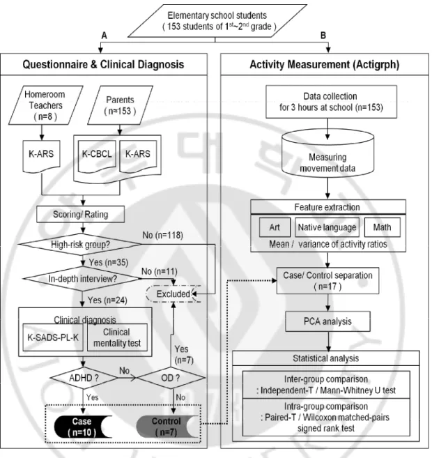
A. Study Overview

To develop objective measures for a definitive characterization of ADHD by monitoring children’s activities at school using an actigraph, new features that reflect children’s activity characteristics were extracted from actigraphic data while they attend school. Based on the extracted activity features, the situational effects of three major courses on the activity of children with/without ADHD were explored. And, a decision support model for ADHD screening was developed.

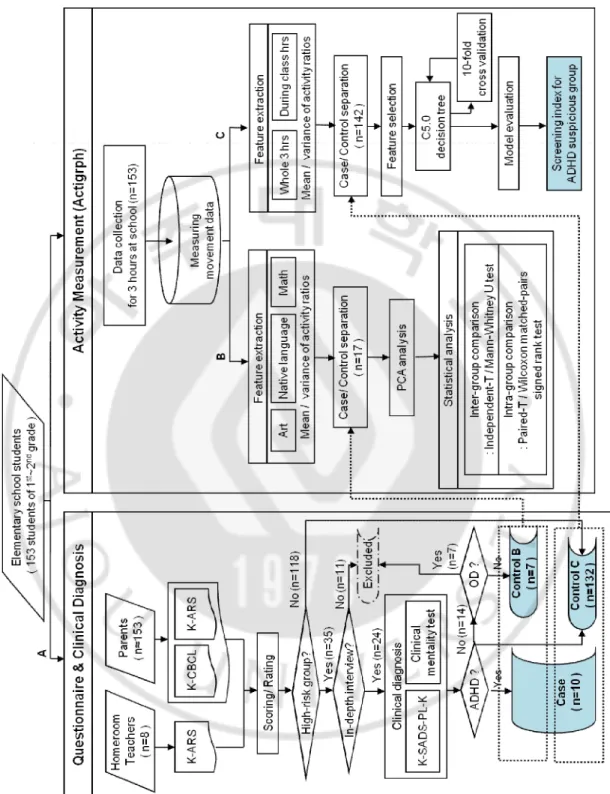
This study was composed of three parts: (1) participant selection from questionnaire administration and clinical confirmation as shown in the (Fig. 1A), (2) exploration on the situational effects on the activity of children with/without ADHD with partitioned activity ranges during three types of classes (art, native language and mathematics), as shown in the in the (Fig. 1B), and (3) development of decision support models for ADHD screening as shown in the (Fig. 1C).

Participant selection (Part A) will be discussed in the following section B. And, the feature extraction and characteristics of the selected case-control subjects (in Parts B and C) will be described in the particular analysis parts in detail.

- 10 -

Fig. 1. Study overview: analysis of activity pattern of children attending elementary school, and development of a screening model for ADHD.

- 11 -

B. Participants

Participants were recruited from a regular elementary school (not a clinic) by screening with questionnaires andtheir parents were provided signed statements of informed consent. The following clinical diagnoses achieved via close examinations and in-depth interviews by child psychiatrists. Those data acquisition was supported by the Ministry of Knowledge Economy’s (MKE) 21st Century Frontier R&D Program, the Ministry of Information and a grant (code #200410) from the Gyeonggi Technology Development Program funded by Gyeonggi Province, Korea.

1. Participants Recruitment and Questionnaires Administration

At first, 153 children (78 boys and 75 girls; mean age, 7.4 ± 0.58 years; range, 6-9 years) were recruited from a local elementary school, in Gyeonggi, South Korea. Questionnaires were administered using the Korean version of the Child Behavior Checklist (K-CBCL) (Oh et al., 1997; Thomas, 1991) and the ADHD Rating Scale-IV (K-ARS) (DuPaul et al., 1998; So et al., 2002) for parents and teachers, after obtaining signed informed consent with a full explanation of the procedures of the study. The CBCL is a widely used tool for the evaluation of various aspects of a child’s behavior, as observed by parents (Thomas, 1991). It consists of a 113-item parent-report questionnaire which assesses the internalizing and externalizing symptomatology of a child. Composed of a total of 18 items, the ARS is designed to evaluate the severity of ADHD symptoms according to the DSM-IV, using a 4-point rating scale ranging from 0 to 3. Generally, the cutoff for a

high-- 12 high--

risk group has been established at a T-score of 63 on the K-CBCL questions and a high score of the upper 10% on the K-ARS (So et al., 2002). In this study, children who scored a T-score of more than 60 on the CBCL questions or who were in the upper 10% on the K-ARS test were selected as the high-risk group.

2.

Participants Selection with Clinical Diagnosis

Children in the high-risk group were interviewed and clinically diagnosed via close examinations and in-depth interviews conducted by four experienced child psychiatrists. As is shown in the (Fig. 1A), each interview included the K-SADS-PL-K (Kiddie-Schedule for Affective Disorder and Schizophrenia-Present and Lifetime Version-Korean Version) (Kim

et al., 2004) and mentality tests. The K-SADS-PL is a semi-structured interview tool

designed to evaluate the severity of ADHD symptoms for 32 different psychiatric disorders in the DSM-IV. The validity and reliability of K-SADS-PL has been verified by its developers. The Korean version of the K-SADS-PL was translated by Kim et al. (2004) and its validity and reliability have been well established for the assessment of ADHD, tic disorders, and oppositional defiant disorder. Additionally, subjects’ Intelligence Quotients (IQ) were also evaluated using a vocabulary test and a block design test included in the Korean-Wechsler Intelligence scale for Children-Third Edition (Kwak, 2001). Among the 35 highly scoring (high-risk) students, 24 children were clinically diagnosed; the other 11 subjects refused to undergo the clinical confirmation process and were therefore excluded from further analysis. Final clinical diagnoses demonstrated that ten of the children had ADHD (ADHD group) and other seven children were normal (non-ADHD group). The other

- 13 -

seven children had psychiatric problems other than ADHD -such as emotional disturbance or tics –; thus, they were excluded from further process steps to evaluate the characteristic influence of ADHD itself. Children diagnosed with ADHD were regarded as gold standards for this study. This was a primary result of ADHD diagnosis: conformation of the ADHD sub-type -such as combined or inattentive type- can be obtained via long-term observation and treatment. Therefore, in this study, the sub-types were not classified. Additionally, those participants were recruited from a general elementary school: prior to our experiment, none of the participants had been diagnosed with or treated for ADHD. All participants were drug-free and had no history of stimulant therapy, both when evaluated and during data collection. None of the subjects had an IQ of less than 80. Hence, none of the participants was considered mentally retarded. As a double-blind test, the diagnoses were not notified to anyone involved in the acquisition of activity data until the end of the experiment (Fig. 1A). This study was approved by the Institutional Review Board of Ajou University Medical Center.

- 14 -

C. Elementary School in Korea

In Korea, children aged from 6 to 12 attended elementary schools of obligation. Children attend 40-minute courses followed by 10-minute recess periods with a standard curriculum including native language, math, science, ethics, art and physical education (plus some additional subjects according to the grades). For the first and second grade students who were the subjects of this study, the first class begins at 9 a.m. and the last (fourth) class ends at 12 p.m. before lunch. In general, children have assigned seats within a classroom, so there is no need to change seats or classrooms except under special conditions. About 30-40 children attend each class with the same teaching materials while sitting in their own assigned seats. One homeroom teacher is assigned to each class, and he or she is wholly responsible for the class.

- 15 -

D. Activity Measurement and Course Information Acquisition

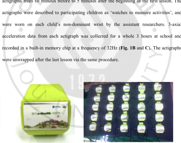
To evaluate the activities of children, an actigraph (LIG Nex1 Co., Ltd., South Korea) shown in (Fig. 2) was placed on each child’s non-dominant wrist from the beginning to the end of the final lesson. Activity data was collected for 1-3 days, for 3 hours per day, during school hours. The actigraphs were managed by four assistant researchers who had been trained in the distribution and management of actigraphs, and the extraction of data: the researchers were divided into groups of two, and went around four classrooms to distribute actigraphs from 10 minutes before to 5 minutes after the beginning of the first lesson. The actigraphs were described to participating children as ‘watches to measure activities’, and were worn on each child’s non-dominant wrist by the assistant researchers. 3-axial acceleration data from each actigraph was collected for a whole 3 hours at school and recorded in a built-in memory chip at a frequency of 32Hz (Fig. 1B and C). The actigraphs were unwrapped after the last lesson via the same procedure.

- 16 -

The children stayed in the same seats of the same classrooms during the measurement periods, and attended all the classes by their own homeroom teachers. Teachers were also responsible for recoding the information about class timetables (the beginning and the end of each course) and the subject information based on a standard elementary school curriculum.

- 17 -

E. Comparisons of Situational Effects on Activity Patterns

1. Overview

In this part of study, comparisons of activity features were conducted between ADHD and non-ADHD groups in order to determine whether the course contents exerted situational influence on the activity distribution of children with ADHD. For that, exploration on the situational effects on the activity of children with/without ADHD was performed with partitioned activity ranges during three types of classes - art, native language and mathematics. The confirmed diagnosed children with ADHD were in the case group, and others -children without ADHD and other psychiatric diseases- were grouped in the control group: group comparisons were performed with partitioned activity regions or activity features by principal component analysis (PCA) and statistical methods (Fig. 3)

- 18 -

Fig. 3. Overview of the study on situational effects on the activity of children with and without ADHD at school. K-ARS: Korean version of the ADHD Rating Scale-IV, K-CBCL: Korean version of Child Behavior Checklist, K-SADS-PL-K: Kiddie-Schedule for Affective Disorder and Schizophrenia-Present and Lifetime Version-Korean Version, OD: Other psychiatric disease (such as emotional disturbance or tic).

- 19 -

2. Feature Extraction

2.1. Activity Features of Partitioned Activity Regions

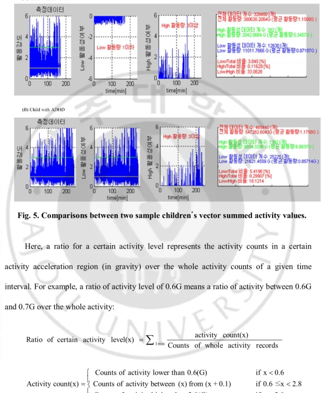
First, vector summed absolute activity (unit: gravity (G)) values were calculated from 3-axial acceleration data measured by actigraphs as shown in (Fig. 4). Comparisons between two sample children’s vector summed absolute activity values are shown in (Fig. 5). Next, activity features such as ratios of mutually exclusive partitioned activity regions (a unit of 0.1G) over the entire activity were extracted in individual 1-minute epochs. Regions from 0.6G to 2.8G (0.1G intervals) and the marginal regions (<0.6G and >2.8G) were considered as shown in (Fig. 6A). The two thresholds for the marginal activity regions were selected from the activity distribution (smaller than 0.1% of total activity).

- 20 -

Fig. 5. Comparisons between two sample children’s vector summed activity values.

Here, a ratio for a certain activity level represents the activity counts in a certain activity acceleration region (in gravity) over the whole activity counts of a given time interval. For example, a ratio of activity level of 0.6G means a ratio of activity between 0.6G and 0.7G over the whole activity:

å

= _1min records activity whole of Counts count(x) activity level(x) activity certain of Ratio 2.8 x if 2.8 x ≤ 0.6 if 0.6 x if 2.8(G) n higher tha activity of Counts 0.1) + (x from (x) between activity of Counts 0.6(G) lower than activity of Counts count(x) Activity ³ < < ï î ï í ì =

- 21 -

From the activity acceleration data, the mean and variance of activity ratios for the middle 14 minutes for each child for each course such as art, native language (Korean) and math were calculated to minimize the influence of recess time.

Fig. 6 . The designed feature extraction process from activity data (I). Activity features such as ratios of mutually exclusive partitioned activity regions (a unit of 0.1G) over the entire activity were extracted in individual 1-minute epochs (Part A). Activity features over a 1.1G threshold were extracted in individual 1-minute epochs (Part B).

- 22 -

2.2. Reproduction of ‘Sum-up Threshold’ Features for Comparison

In addition to the newly introduced activity features, the previously-employed activity features – summed activity counts over a certain threshold – were included to make comparisons between the features. The criterion threshold for activity was established: activity counts above the defined threshold were summed into mean and variance via the same 1-minute epoch as new features.

The previously used activity feature (hereafter, ‘sum-up threshold’ feature) was reproduced, based on several previous studies (Dane et al., 2000; Gruber et al., 2006; Halperin et al., 2003; Porrino et al., 1983; Schwartz et al., 2004; Swanson et al., 2002; Tsujii

et al., 2007) in which ADHD and non-ADHD groups were compared using actigraphs, and

the instruments, experimental settings, placement of the actigraphs, time period and obtained data were mentioned. All the actigraphs employed in the previous studies were not the same; generally speaking, they measured the counts (or time-above threshold) according to the basic setting option of a 0.01G threshold with a zero crossing mode (ZCM) and the summed counts (or time period) were stored within a 1-min epoch. Although there were some differences among several actigraphs, including frequencies of measurements and sensitivity, the calculated counts were converted into activity ratio above the threshold rather than the mere counts, as an extension of our proposed features and activity ratios.

In the most of the previous studies, the thresholds of the actigraph were 0.01G (Teicher, 1995; Teicher et al., 1996; Tsujii et al., 2007) or 0.02G (Swanson et al., 2002) as

- 23 -

basic settings. In our data, all the collected activity data were above 0.01G: this indicates that the sensitivity (or threshold) should be adjusted according to the actigraphs and the relevant attachment positions. Because no previous study has provided the portion of above-threshold activity (counts) over the whole range of activity, it proved difficult to establish a threshold with the same effect. With the actigraph that was used in this study, activities larger than 1.0G took a 90% (on average) portion of the whole activities; activities greater than 1.2G were 10-20% with a sharp decline. In the case of 1.1G, the activities accounted for 43-51% of the whole range of activity. Additionally, the mean activity values of each group were 1.10G (non-ADHD) and 1.15G (ADHD): the threshold was set to 1.1G and extracted the means/variances of activity counts with 1-min epochs (shown in (Fig. 6B)).

3. Principal Component Analysis (PCA)

Prior to statistical evaluation of whether or not the features proposed (48 partitioned activity ratios) were reflective of different situational influences on the activity of children with and without ADHD, principal component analysis (PCA) was employed to evaluate the resolving power of the selected most informative feature set among the high-dimensional features for children with and without ADHD. PCA (also referred to as the Karhunen-Loeve, or K-L method) is a data compression and visualization method: The original k-dimensional data were projected onto a much smaller space by k-dimensional orthogonal vectors without loss of much information. Therefore, PCA can be utilized as a form of dimensionality reduction (Han & Kamber, 2001). This involves a mathematical procedure in which a

- 24 -

number of possibly correlated variables are transformed into a smaller number of uncorrelated variables –which are referred to as principal components. The first principal component explains as much as possible of the variability in the data, and each succeeding component also explains as much as possible of the remaining variability (Witten & Frank, 2005). In this study, three principal components were employed. Based on the 48 series of calculated activity features -the mean or variance of activity acceleration (determined by summing up the absolute vector data from 3-axial accelerometer)-, each child represented as a point in a 48-dimensional data space for each course. Next, using the PCA analysis in MATLAB (R2007a, MathWorks Inc., MA), all 17 of the children (10 ADHD and 7 non- ADHD) with their individual feature vectors– composed of principal components 1, 2 and 3 -were placed in a three-dimensional principal component space. The data points, which -were located close to one another on the 3-dimensional graph, had similar characteristic: similar components were found by analyzing the grouping or alignment patterns among the distributed data points. Finally, the smallest ovals were drawn necessary to include all the members of individual classes (ADHD and non-ADHD) in each case, and compared them to determine whether or not the ADHD and non-ADHD groups were separable.

- 25 -

4. Statistical Analysis

All the activity data in each situation was compared as follows: (1) to compare the activity differences between the ADHD and non-ADHD groups, independent-t test or Mann-Whitney U-tests were separately applied in different course environments (Lehmann, 1975); and (2) to compare activity difference within each group, paired course comparisons were conducted via paired-T test or Wilcoxon matched-pairs signed rank test (Milton & Arnold, 2004), according to the Shapiro-Wilk normality test. In the case of sum-up threshold features, a new normality test was conducted after log transformation, if the normality hypothesis was not satisfied; in the case of new features, owing to the incapability due to zero data values in some sections, non-parametric analyses were conducted if the raw data did not satisfied the normality hypothesis. For both cases, p-values of < 0.05 were considered as statistically significant (with the SPSS 15.0, a Korean version).

- 26 -

F. Model Construction for ADHD Screening

1. Overview of Model Construction

The principal objective of this study part was to develop a decision support model for ADHD screening by monitoring children’s activities at school using a 3-axial accelerator (actigraph). The confirmed diagnosed children with ADHD were in the case group, and all the other children were grouped in the control group as children without ADHD. Two decision tree models were constructed using the C5.0 algorithm: [A] from whole hours (class + playtime) and [B] during classes. Accuracy, sensitivity, and specificity were evaluated. Positive predictive value (PPV), negative predictive value (NPV), odds ratio (OR), relative risk (RR), likelihood ratio (LR +/-) and area under ROC curve (AUC) were also calculated for evaluation (Fig. 7).

The primary results of this model construction for ADHD screening was published in the Applied Clinical Informatics (Kam et al., 2010)

- 27 -

Fig. 7. Overview of the Process-flow for ADHD screening model construction: (A) a general process for screening & diagnosis of ADHD and (B) process to build screening models for ADHD with activity features. *: dropped from further clinical confirmation, K-ARS: Korean version of the ADHD Rating Scale-IV, K-CBCL: Korean version of Child Behavior Checklist, K-SADS-PL-K: Kiddie-Schedule for Affective Disorder and Schizophrenia-Present and Lifetime Version-Korean Version.

- 28 -

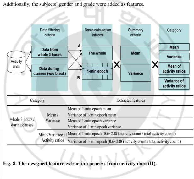
2. Feature Extraction and Selection

2.1. Feature Extraction

From the data acquired over the 1-3-day collection period, data from the first valid day was taken for each student. Vector-summed absolute activity values (unit: gravity (G)) were calculated from the 3-axial activity data. Afterward, the same as the feature extraction for class comparison experiment, the following overall (Fig. 8A) and 1-minute epoch features (Fig. 8B) were extracted: activity features such as ratios of mutually exclusive partitioned activity regions (a unit of 0.1G) over the entire activity were extracted in individual 1-minute epochs. Regions from 0.6G to 2.8G (0.1G intervals) and the marginal regions (<0.6G and >2.8G) were considered. The two thresholds for the marginal activity regions were selected from the activity distribution (smaller than 0.1% of total activity). Here, a ratio for a certain activity level represents the activity counts in a certain activity acceleration region (in gravity) over the whole activity counts of a given time interval. For example, a ratio of activity level of 0.6G means a ratio of activity between 0.6G and 0.7G over the whole activity:

å

= _1min records activity whole of Counts count(x) activity level(x) activity certain of Ratio 2.8 x if 2.8 x ≤ 0.6 if 0.6 x if 2.8(G) n higher tha activity of Counts 0.1) + (x from (x) between activity of Counts 0.6(G) lower than activity of Counts count(x) Activity ³ < < ï î ï í ì =

- 29 -

The features were assigned to one of two categories: (1) features from the whole three hours (class + playtime) and (2) features during classes. That is to say, ‘whole three hours’ means that the object of analysis was data was obtained all along the three measuring time. The term, ‘during classes’, refers specifically to the middle 14 minutes of each class. Additionally, the subjects’ gender and grade were added as features.

Fig. 8. The designed feature extraction process from activity data (II).

The same as the feature extraction for class comparison experiment, the following overall (Part A) and 1-minute epoch features (Part B) were extracted.

- 30 - 2.2. Feature Selection

The numbers of primarily extracted features were 104 (52 for each category), which reached almost one-third of the number of subjects to be classified (n=153). Relatively high number of features compared with that of samples can cause a problem, ‘curse of dimensionality’: it gets harder to analysis data as the dimension of data is getting bigger. Especially in case of classification, because data gradually becomes rare in the data space as the dimension increases, it is difficult to construct a trustful classifier for all the possible samples (subjects). As a result, the accuracy of classification is getting lower with high-dimensional data. Therefore, the number of selected features was dependent on the number of samples (Yun et al., 2007) -in our case, the number of children reflected in a model construction (Tan et al., 2006).

There are many benefits that can be obtained from a dimension reduction. The core advantage is that many data mining algorithms work better in lower data dimension –the number of data attributes. One reason is that dimension reductions remove un-related features and noises; and also it solves the curse of dimensionality. Another benefit is that the dimension reduction creates models with smaller number of attributes (features), and makes better understandable ones. Additionally, it also makes easier data visualizations. Lastly, it has an effect on reducing the time and memory required by data mining algorithms.

Though there are many kinds of methodologies for dimension reduction (Witten et al., 2005), WEKA (WEKA 3.6, University of Waikato Hamilton, New Zealand) software and three of its feature selection options were used for feature selection process. Firstly, the ranker search method was utilized: it ranks features in conjunction with information gain

- 31 -

attribute evaluator, and calculates the relative worth of attributes by measuring the information gain with respect to the class. The upper 20 highly ranked features were selected by 10-fold cross-validation. Secondly, the BestFirst (forward) feature selection method was used: it searches the space of attribute subsets by greedy hill-climbing segmented with a backtracking facility, starting with the empty set of attributes and search forward. With CfsSubset evaluator, the BestFirst method calculates the worth of subsets of attributes by considering the individual predictive ability of each feature along with the degree of redundancy between them. Features were selected that were picked out more than once by 10-fold cross-validation. Lastly, a genetic search method combined with CfsSubset evaluator was utilized. With a genetic algorithm that is used in the Genetic search method, features were selected that were picked out more than twice by 10-fold cross-validation with setting of random seed and no start set. Other variable options of each search method and evaluator were set as default in WEKA. And, the union combination of selected features from three methods was selected as the final feature set.

- 32 -

3. Decision Tree Model Construction for ADHD Screening

3.1. Introduction of Decision Tree Methodology

A decision tree is a supervised classification method exploited in data mining; decision trees are used to categorize subjects into pre-established classes. First, a decision tree is constructed using a ‘training’ set of subjects. Then, the constructed model can be utilized as a predictive decision-support model for new subjects. A decision tree has a flowchart-like upside-down tree structure (Han & Kamber, 2001), in which dependent variables are positioned at the lowest ends of the tree. In this study, the dependent variable is whether or not a subject is in the high-risk group of ADHD. Nodes are formed when the branches stretch down, where selected features–such as independent variables in regression-and conditions for the features are placed. The selected features or conditions represent the best capability to separate the subjects gathered at a node into their own dependent variable, as compared with other features or conditions. More than two down-stretching branches can extend from a node. Following down the very branches that satisfy each condition at every node encountered, it reaches a lowermost node with a final decision as to whether or not the unidentified subject who travels with us is at high risk for ADHD. After model construction, a decision tree lists several features and conditions of subjects by which subjects can be divided into proper dependent variables (ADHD and non-ADHD), and it shows the conditions schematically.

- 33 - 3.2. Various Decision Tree Algorithms

Theoretically, there are exponentially many decision trees that can be formed by any combination of a given set of attributes (features). Finding the optimal decision tree is a NP-complete problem; so, many algorithms utilized heuristic search methods in hypothesis spaces. In general, many of those algorithms use greedy strategy, a top-down and divide-and –conquer strategy for choosing features to divide a given data set, to breed a decision tree by making serial optimal decisions (Tan et al., 2006).There are many statistical algorithms and commercial software are available for the construction of a decision tree. And, they have been developed based on two main techniques: depth-first (Hunt’s method) and breadth-first greedy technique (Matthew & Sajjan, 2009). Matthew et al. have performed a comparison study on various decision tree algorithms that have been used in many literatures for solving problems related to practical classifications. Among them, the most frequently used algorithms such as IDE3 (Iterative Dichotomiser 3), C.4.5/C5.0, CART (classification and regression trees) and SPRINT were considered as candidates for the most proper decision tree algorithm on ADHD screening.

Matthew et al. have compared classification accuracies of the four mentioned algorithms with a variety of class size (from 2 to 13), attribute number (from 9 to 24) and record number (from 270 to 43,499): SPRINT classifier showed the best classification accuracy among all the classifier, and C4.5 was the following with difference of 0.5%-1.63%. In cases of IDE3 and CART, the resulting accuracies were rather lower. And, the variance of the accuracies was heavy according to class size, attribute number and record number. On

- 34 -

the contrary, in SPRINT and C4.5, the conditions did not affect the classification accuracy (Matthew & Sajjan, 2009). SPINT is specially designed for a massive data handling, and provides extendable parallel algorithm. However, that function was not compulsory for the targeting ADHD screening; in this study, C5.0 algorithm which is the commercial successor of and well-known classifier.

3.3. Applied Decision Tree Algorithm: C5.0 Algorithm

C5.0 offers a number of improvements on C4.5 (Rulequest research, 2009). Especially in the aspect of resulting performance, C5.0 gains similar results compared to C4.5, with considerably smaller decision trees. To avoid errors that are caused by model over-fitting, simpler – less complicated- models are preferred: this is called Occam’s razor or principal of parsimony (Tan et al., 2006). And, the class imbalance problem of the subject groups, which will be discussed in the following section, was resolved by the un-equal misclassification costs. C5.0 provides newly adapted weighting function of variable misclassification cost, and that is another reason for choosing C5.0 algorithm.

Two tree-shaped screening models were constructed using the C5.0 algorithm (Clementine 10.1, SPSS Inc.) according to two groups of features: (1) from whole hours (class+playtime) – Model A and (2) during classes – Model B. C5.0 constructs decision trees based on the concept of Information Entropy, and assesses the normalized information gain (differences in entropy) that results from the selection of a valuable feature for the separation

- 35 -

of the subjects into groups (ADHD and non-ADHD). The feature with the highest normalized information gain is the one employed in the decision regarding the downward-stretching branches. The algorithm subsequently recurs on the smaller subset of subjects, thereby resulting in a tree-shaped model (Quinlan, 1993).

3.4. Avoiding Model Over-fitting

To avoid over-fitting of models during model construction steps, local and global pruning were applied. Pruning prevents the formation of too complex sub-trees that result in over-fitting toward train data: this is utilized to overcome the over-fitting problem. Too high threshold produces under-fit models; on the contrary, too low threshold may not be enough to overcome the over-fitting problem. In Clementine 12.0, options for pruning can be set: (1) severity setting for local pruning, which examines sub-trees and collapses branches to increase the accuracy of the model and (2) setting for global pruning that collapses weak sub-tree from the global view as explained at the Clementine documentation.

- 36 -

4. Solving Class Imbalance Problem

As is the cases in many other clinical environments, there exists a group imbalance problem: the non-ADHD group was represented by a large number of examples, whereas the ADHD patient group was represented by only a few examples. There are many approaches to addressing the group imbalance issue, and they can be divided into two type. One is sampling: it changes the distribution of data cases, and makes the fewer group more representative in the training data set (Tan et al., 2006). The other one is cost-sensitive methodology by adjusting the misclassification costs.

In the sampling methodology, there are two methods: under-sampling and over-sampling. Under-sampling randomly selects small fraction of cases of the members from the majority group to make up a proper sized group compared to the other minority group. The problem of under-sampling is that several useful cases in the majority group are excluded from training data set, and result in an un-optimized model.

On the contrast, over-sampling duplicates several-folds of cases of the members from the minority group to make up the same size of group compared to the other majority group. Over-sampling may provides abundant cases that guarantee the necessary boundaries for classification. However, it also falls into model over-fitting problem because of the duplicated noises from noisy data. Theoretically, over-sampling does not supply any new information on the training set: the replications of case only perform a limited role that protects a certain part of regions represented by vary few cases (Tan et al., 2006).

The second method is cost-sensitive methodology by adjusting the misclassification costs. In some contexts, certain kinds of errors are more costly than others. For example, it

- 37 -

may be more costly to classify a child with ADHD as a normal than it is to classify a normal child as a patient with ADHD. The misclassification cost was applied, by altering the relative importance of different kinds of prediction errors as costs of misclassification of the small and the large classes (Japkowicz & Stephen, 2002).

The applied cost of misclassification of an ADHD patient (as children without ADHD) was 13.2 times higher than the misclassification cost of a child without ADHD. The cost was applied in accordance with the imbalance of ADHD/non-ADHD class (1:13.2), and was reflective of the relative importance of screening children with ADHD from children without ADHD, considering the social costs that must be shouldered when proper opportunities for treatment are lost. There also can be inverse cost by mis-screening a normal child as a ADHD patient. However, the result of classification is used for the purpose of screening, not for diagnosis; the cost for medical consultation may be the only inverse cost. And, that cost did not considered in this study.

- 38 -

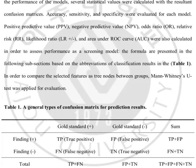
5. Model Evaluation and Statistical Analysis

In constructing the models, 10-fold cross-validation methodology was utilized that made it possible to utilize all observations as training and validation, and each of these observations was used for validation exactly once (Quinlan, 1993). (Fig. 1C). To evaluate the performance of the models, several statistical values were calculated with the resultant confusion matrices. Accuracy, sensitivity, and specificity were evaluated for each model. Positive predictive value (PPV), negative predictive value (NPV), odds ratio (OR), relative risk (RR), likelihood ratio (LR +/-), and area under ROC curve (AUC) were also calculated in order to assess performance as a screening model: the formula are presented in the following sub-sections based on the abbreviations of classification results in the (Table 1). In order to compare the selected features as tree nodes between groups, Mann-Whitney’s U-test was applied for evaluation.

Table 1. A general types of confusion matrix for prediction results.

Gold standard (+) Gold standard (-) Sum

Finding (+) TP (True positive) FP (False positive) TP+FP

Finding (-) FN (False negative) TN (True negative) FN+TN

- 39 - 5.1. Accuracy

The accuracy means the ability to discriminate a child without ADHD (gold standard (-)) as a member of ‘Non-ADHD’ (Finding (-)) group and a child with ADHD (gold standard (+)) as a member of ‘ADHD’ (finding (+)) group. That is, it is the proportion of true results (both TN and TP) in the population.

Accuracy = _{(TP + FP + TN + FN)}(TP + TN)

5.2. Sensitivity and Specificity

Sensitivity means the ability to discriminate children with ADHD (gold standard (+)) as an ‘ADHD’ (finding (+)).

Sensitivity = _{(TP + FN)}TP

And, specificity means the ability to discriminate children without ADHD (gold standard (-)) as a ‘non-ADHD’ (finding (-)).

- 40 - 5.3. PPV and NPV

The positive predictive value (PPV), or precision rate, is the proportion of children with positive screening result (finding (+)) who are correctly diagnosed as children with ADHD.

PPV = _{(TP + FP)}TP

Alternatively, the negative predictive value (NPV) is the proportion of children with negative screening result (‘non-ADHD’) who are correctly diagnosed as children without ADHD.

NPV = _{(FN + TN)}TN

However, the value of PPV and NPV depend on the prevalence of ADHD. Therefore, they can be calculated as followed, with consideration of the prevalence rate.

PPV = _{(sensitivity x prevalence rate) + {(1 − speci icity)(1 − prevalence rate)}}sensitivity x prevalence rate

- 41 - 5.4. Odds Ratio (OR)

The odds ratio is a measure of effect size, and is the odds of the occurrence of finding (+) in the gold standard (+) group to the odds of it occurring in the gold standard (-) group.

OR = TP FP FN TN = TP x TN_{FP x FN} 5.5. Relative Risk (RR)

Relative risk is a ratio of the probability of the occurrence of gold standard (+) in the finding (+) group versus the finding (-) group.

RR = TP (TP + FP) FN (FN + TN) 5.6. Likelihood Ratio (LR)

Likelihood ratio incorporates both the sensitivity and specificity of the test and provides a direct estimate of how much a test result will change the odds of having a disease. That means the descriptive power of the screening model. The likelihood ratio for a positive result (LR+) tells you how much the odds of ADHD increase when the prediction of decision tree model is positive. The likelihood ratio for a negative result (LR-) tells how much the odds of ADHD decrease when the prediction is negative. Likelihood ratio is not affected by the changes of prevalence rate, and more stable to them than sensitivity and specificity.

- 42 -

LR (+) = _{1 − speci icity}sensitivity LR (−) = 1 − sensitivity_{speci icity}

5.6. AUC

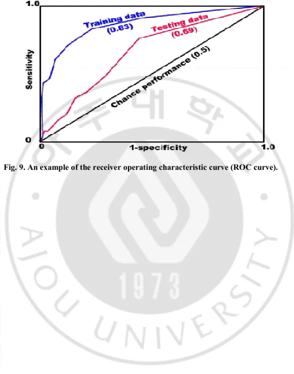
To avoid having to select a single threshold for classification, one may scan through all possible thresholds, and observe the effect on the true positive rate (sensitivity) and the false positive rate (1-specificity). Graphed as coordinate pairs, these measures form the receiver operating characteristic curve (or ROC curve, for short). The ROC curve describes the performance of a model across the entire range of classification thresholds. Every ROC curves start from the bottom-left corner, and be drawn to the top-right corner as shown in (Fig. 9), moving along the ROC curve represents trading off false positives for false negatives. Generally, random models will run up the diagonal, and the more the ROC curve bulges toward the top-left corner, the better the model separates the target class from the background class.

If one is not interested in a specific trade-off between true positive rate and false positive rate (that is, a particular point on the ROC curve), the AUC (Area under ROC curve) is useful in that it aggregates performance across the entire range of trade-offs. And, the wider AUC means the better diagnostic or screening method.

- 43 -

- 44 -

III. RESULTS

A. Comparisons of Activity Patterns

1. Participant Selection

Via the process of screening and diagnosis of children with and without ADHD (Fig. 1A), our group comparisons were conducted with 10 children with ADHD (eight boys and two girls; mean age, 7.2 ± 0.63 years; range, 6-8 years) and seven children without ADHD (six boys and one girl; mean age, 7.6 ± 0.53 years; range, 7-8 years) as shown in (Table 2). Initial rating scale data as well as other demographic information (age and gender) is shown in (Table 3), coupled with t-tests of potential between-group differences.

Table 2. Results of systematic questionnaire and clinical confirmation. Systematic questionnaire

& clinical confirmation

Systematic questionnaire

only Total

ADHD Other disease Normal High-risk Low-risk

Female 2 1 6 3 63 75

Male 8 6 1 8 55 78