Minimum Hellinger Distance Estimation and Minimum Density Power Divergence Estimation in Estimating Mixture Proportions

2005, Vol. 16, No. 4, pp. 1159∼1165

Minimum Hellinger Distance Estimation and Minimum Density Power Divergence Estimation in Estimating

Mixture Proportions

Ro Jin Pak

Abstract

Basu et al. (1998) proposed a new density-based estimator, called the minimum density power divergence estimator (MDPDE), which avoid the use of nonparametric density estimation and associated complication such as bandwidth selection. Woodward et al. (1995) examined the minimum Hellinger distance estimator (MHDE), proposed by Beran (1977), in the case of estimation of the mixture proportion in the mixture of two normals. In this article, we introduce the MDPDE for a mixture proportion, and show that both the MDPDE and the MHDE have the same asymptotic distribution at a model. Simulation study identifies some cases where the MHDE is consistently better than the MDPDE in terms of bias.

Keywords : Bias, Density power divergence, Hellinger distance

1. Introduction

Robustness procedures typically obtain robustness at the expense of not being optimal at the true model. However, Beran (1977) has suggested the use of the MHDE which has certain robustness properties and is asymptotically efficient at the true model. The theories about MHDE have been studied by many researchers like Tamura and Boos (1986) (discussed the estimation of location and covariance in multivariate data), Eslinger and Woodward (1991) (discussed the estimation of the parameters of the normal distribution with unknown location and scale).

Woodward et al. (1995) discussed MHD estimation in the case of estimating the

1) Associate Professor, Division of Information and Computer Sciences, Dankook University, Seoul, Korea.

E-mail: [email protected]

mixture proportion of the mixture of two normals, and showed that the MHDE were robust and obtained full efficiency at the true model.

Suppose X

, …,X

being i.i.d. with a distribution G with corresponding density g and consider f

(x) = (1- θ) f

(x)+ θf

(x), where f

and f

are distinct, continuous densities on R, and θ∈ [ 0, 1]. If ˆ g

n

is a Hellinger consistent density estimator for f

, then Woodward et al. (1995) provided a very important theorem which concluded with the asymptotic statement at the model about the estimator ˆ θ

n

for the mixture proportion θ;

n( θ ˆ

n

- θ - B

)→N( 0,I( θ)

), (1.1) where I( θ) is the Fisher information matrix and B

is given by

B

= 2C

⌠

⌡ψ

f

( ˜ g

- f

) and C

→1 in probability

with E[ g ˆ

n

] = g ˜

n

. and ψ

= 1 I( θ)

f

- f

f

.

The above result actually was built upon the Theorem 4.1 by Tamura and Boos (1986) discussing the asymptotic distribution of the estimators for multivariate location and covariance. A kernel density estimator is a usual choice for ˆ g

n

as

ˆ g

n

(x) = 1

n ∑ _h ^{1 k} ( ^{x - X h}

)

with a kernel k( ⋅) and a bandwidth h. We have ˜ g

n

→f

at the model g = f, as h→0, nh→∞, then B

→0.

Applying the MHDE to the real data associates complications such as bandwidth selection. There has been no reliable study about how to select bandwidths in this case. Meanwhile, Basu et al. (1998) proposed a class of ' density power divergences' indexed by a single parameter, α, which controls the trade-off between robustness and efficiency estimation. A good news is that in the process of estimation a density estimator is not required , that is, there is no need to select a bandwidth.

Consider a parametric family of models { F

}, indexed by the unknown

finite-dimensional parameter θ in an open connected subset Ω of a suitable

Euclidean space, possessing densities { f

} with respect to Lebesque measure. Let

G be the distribution underlying the data, having density g with respect to the

same measure. Basu et al. (1998) define the density power divergence between g and f

to be

d

(g, f

) = ⌠ ⌡ { ^f

^- ( ^{1 + 1 α} ) ^gf

^{+ 1 α g}

} dz ( α > 0), d

(g, f

) = lim

α→0

d

(g, f

) = ⌠ ⌡g log ( g/f

) dz.

We shall frequently use the shorthand notation d

',d

'',… for the derivatives of d

with respect to θ. Note that d

(g, f

) is the Kullback-Leiber divergence.

The resulting sample minimum density power divergence estimators are those values ˆ θ

α

generated by minimizing

⌠ ⌡f

dz - ( 1 + 1

α )n

∑

i = 1

f

(X

)

with respect to θ, when α > 0, and the negative loglikelihood

∑

n

i = 1logfθ(Xi)

when α = 0. It can be checked easily that the estimating

equations have the form

n

∑

i = 1

f

(X

)u

(X

)- ⌠ ⌡ f

u

dz,

where u

(z) = ∂ log f

(z)/∂ θ is the maximum likelihood score function. Note that this estimating equation is unbiased when g= f

.

In this article we consider the MDPDE for a mixture proportion and we show that both the MDPDE and the MHDE have the same asymptotic distribution at a model. However, simulation study identifies some cases where the MHDE is better than the MDPDE in terms of bias.

2. Asymptotic properties of the MDPDE for the mixture proportion

Consider the estimation of the proportions θ

, θ

, …,θ

in the mixture density f( x) = θ

f

(x) + θ

f

(x) + … + θ

f

(x).

Definition 1: Let X

, …,X

be i.i.d. with a distribution G with

corresponding density g, that depends on θ = ( θ

, …,θ

), the minimum density power divergence estimator for the mixture proportion ˆ , generated by the θ quantity minimising

d

(f

) = ⌠ ⌡f

dz - ( 1 + 1

α )n

∑

n

i = 1

f

(X

) (1.2) with respect to θ for a given α∈( 0, 1].

Theorem 1: Let X

, …,X

be i.i.d. with a distribution that depends on θ = ( θ

, …,θ

). Under certain regularity conditions, given Basu et al. (1997), there exists ˆ such that, as n→∞, θ ˆ θ

n

is consistent for θ, and n

( θ ˆ

n

- θ) is asymptotically multivariate normal with (vector) mean zero and covariance matrix J

K J

, where J and K are given by

J = ⌠ ⌡u

(z)u

(z)f

dz + ⌠ ⌡i

(z) - αu

(z)u

(z) g( z) - f

(z) f

(z)dz, K = ⌠ ⌡u

(z)u

(z)f

(z)g(z)dz - ξξ

with ξ = ⌠ ⌡u

(z)f

(z)g(z)dz , where u

(z) = ∂ log f

(z)/∂t.

Proof: For estimator ˆ θ

n

and the true value θ

, by Taylor series expansion of d

(f

) in (1.2), we have

n( θ ˆ

n

- θ

) = ( 1 / n)d

'(f

) - ( 1/n)d

''(f

)- (1/2n)( θ ˆ

n

- θ)d

'''(f

) |

, where θ

lies between θ

and ˆ θ

n

. Consider first the numerator, and then by the CLT

1

1 + α d'

(f

) = ⌠ ⌡f

(z)f

'(z)dz - n

∑

i = 1

f

(z)f

'(z)

= ⌠ ⌡f

(z)u

(z) - n

∑

n

i = 1

f

(z)u

(z)

→ N( 0, K).

In the denominator the consistency of the estimator, assumption of boundness of

d'''

(f

) and law of large numbers give - ( 1/n)d''

(f

)→ J. The constant

( 1 + α) will be cancelled off. Proof is rather straight forward if we follow closely

the proof of Theorem 6.4.1 of Lehmann (1983) (which is for the maximum

likelihood estimator) with appropriate modifications to cope with density power divergence. The formulae look complicated, but let d

(f

) play like L( θ) in the proof of Lehmann (1983).

Suppose that the true distribution g belongs to the parametric family { f

}.

Then the formular for J, K and ξ simplify to

J = ⌠ ⌡u

(z)u

(z)f

(z)dz,

K = ⌠ ⌡u

(z)u

(z)f

(z)dz- ξ ξ

with ξ = ⌠ ⌡u

(z)f

(z)dz.

Note that, in the limit α→0, J and K both become equal to the Fisher information matrix I(θ)

. This asymptotic result at the model is the same as the one in (1.1) by Woodward et al. (1995) with f

= (1- θ) f

+ θ f

.

3. Finite sample properties

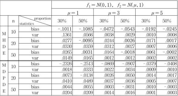
We showed that both the MDPDE and the MHDE have the same asymptotic distribution under certain conditions. In order to verify the asymptotic equivalence, simulations were carried out with 500 random samples of sizes, 10, 20 and 50, generated from 30% and 50% mixtures of two normals, N( 0, 1) and

N( 1, 1), N( 3, 1), N( 5, 1), respectively. An Epanechnikov kernel and a

bandwidth by 'bandwidth.nrd' of S-plus (Venables and Ripley, 1996) are used for

a density estimator. Basu, et al. (1998) did not provide no universal way of

selecting an appropriate α parameter, but recommended α near 0.25. For

computational convenience α = 1/3 is used for MDPDE, In the course of

verifying the above theory we have discovered the case where the MHDE is

consistently better than the MDPDE in terms of having smaller bias. The results

are in Table 1; the numbers in bold indicate the cases where the absolute value

of the bias of the MHDE is smaller than that of the MDPDE, where n = 10 or

proportion is 50%. The variances of both estimators are very close, but there is

no systematic pattern in sizes like biases. The one thing we can think of at this

moment is that this phenomenon is related with the closeness of the model f and

the true density g, because unbiasedness of both the MHDE and the MDPDE is

attained under the condition that g = f. In practice the true density g should be

estimated. Recall that g is estimated by an empirical density for the MDPDE and

by an smoothed (kernel) density estimator for the MHDE. When a kernel density

estimator is more effective in estimating g than an empirical density, we expect

that bias of the MHDE would be smaller than that of the MDPDE.

4. Conclusions

We show that the MDPDE and the MHDE have the same asymptotic distribution when estimating mixture proportions. The MDPDE performs quite well without worrying about choosing a smoothing parameter, however we could identify the cases where the size of bias of the MHDE is smaller than that of the MDPDE are identified. We need more thorough investigation why it happens, but at this moment we conclude that there are cases where smoothing data with a kernel function in estimating a mixture proportion is useful in reducing bias.

Table 1. Statistics on the estimates of mixture proportions ; f= (1-θ)f

+ θf

f

= N(0,1), f

= N( μ, 1)

μ = 1 μ = 3 μ = 5

n

statistics

30% 50% 30% 50% 30% 50%

M H D E

10 bias -.1011 -.1085 -.0472 -.0543 -.0192 -.0245

var .1361 .0566 .0038 .0029 .0010 .0008

20 bias .0277 -.0095 .0244 .0026 .0171 .0017

var .0330 .0359 .0312 .0027 .0007 .0006

50 bias .0265 .0031 .0164 -.0018 .0061 -.0002

var .0149 .0165 .0012 .0012 .0002 .0002

M D P D E

10 bias -.2326 -.2513 -.0869 -.0907 -.0379 -.0408

var .0018 .0333 .0022 .0034 .0009 .0010

20 bias .0073 -.0138 .0026 .0050 .0014 .0017

var .0410 .0489 .0037 .0036 .0005 .0007

50 bias .0044 .0055 .0003 -.0031 .0010 -.0003

var .0204 .0209 .0014 .0016 .0001 .0003

References

1. Basu, A., Harris, I., Hjort, N., and Jones, M. (1995), Robust and efficient estimation by minimizing a density power divergence, Biometrika, 85, 549-559.

2. Beran, R. (1977), Minimum Hellinger distance estimates for parametric models, The Annals of Statistics, 5, 445-463.

3. Eslinger, P. and Woodward, W. (1991), Minimum distance estimation for normal models, Journal of Statistical Computation and Simulation, 39, 95-114.

4. Lehman, E. L. (1983), Theory of Point Estimation, Wiley, New York.

5. Tamura, R. and Boos, D. (1986), Minimum Hellinger distance estimation for multivariate location and covariance, Journal of the American Statistical Association, 81, 223-229.

6. Woodward, W., Whitney, P. and Eslinger, P. (1995), Minimum Hellinger distance estimation of mixture proportions, Journal of Statistical

Planning and Inference, 48, 303-319.

7. Venables, W. and Ripley, B. (1996), Modern Applied statistics with S-Plus, Springer, New York.

[ received date : Oct 2005, accepted date : Nov. 2005 ]