Numerical Analysis of Turbulent Combustion and Emissions in an HRSG System

Manuscript received on May 10, 2019, Accepted on July 15, 2019

1 KEPCO Research Institute, Korea Electric Power Corporation, 105 Munji-ro Yuseong-gu, Daejeon 34056, Korea

2 Pohang University of Science and Technology, Pohang, Gyeongbuk 790-784, Korea

† [email protected]

Numerical Analysis of Turbulent Combustion and Emissions in an HRSG System

가스터빈 열 회수 증기 발생기의 난류연소 해석과 배기가스 예측 및 검증

Jihoon Jang

, Karam Han

, Hoyoung Park

, Wook-Ryun Lee

, Kangyul Huh

장지훈

, 한가람

, 박호영

, 이욱륜

, 허강열

Abstract

The combined cycle plant is an integration of gas turbine and steam turbine, combining the advantages of both cycles. It recovers the heat energy from gas turbine exhaust to use it to generate steam. The heat recovery steam generator plays a crucial role in combined cycle plants, providing the link between the gas turbine and the steam turbine. Simulation of the performance of the HRSG is required to study its effect on the entire cycle and system. Computational fluid dynamics has potential to become a useful to validate the performance of the HRSG. In this study a solver has been implemented in the open source code, OpenFOAM, for combustion simulation in the heat recovery steam generator. The solver is based on the steady laminar flamelet model to simulate detailed chemical reaction mechanism. Thereafter, the solver is used for simulation of HRSG system. Three cases with varying fuel injections and gas turbine exhaust gas flow rates were simulated and the results were compared with measurements at the system outlet. Predicted temperature and emissions and those from measurements showed the same trend and in quantitative agreement.

Keywords: Computational Fluid Dynamics, CFD, Turbulent Combustion, Steady Laminar Flamelet Model, Heat Recovery Steam Generator, HRSG

I. INTRODUCTION

Heat Recovery Steam Generator (HRSG) is the main components of a combined cycle power plants which used in a wide range of power generation applications due to high efficiency and positive effect on plant flexibility. The reason that favors the use of combined cycle plants is its ability to use low carbon content fuels and its low impact on the environment. The drawback in using a simple gas turbine cycle is that the exhaust temperature is high. The maximum efficiency of a simple gas turbine cycle is around 35% [1].

Whereas, the efficiency of the simple cycle system can be increased by recovering some of the heat energy carried away by the exhaust gas from the gas turbine and generating steam in a HRSG system. It forms the heart of the combined cycle and

its performance has a direct impact on the overall efficiency of the combined cycle system. Therefore, optimal design of HRSG through numerical analysis is an important issue due to the increase in fuel prices and decrease in fossil fuel resources.

A simulation of the performance of the HRSG is required to

study its effect on the entire system. It is clear that CFD has

the potential to become a useful to validate the performance

of the HRSG, the successful application of CFD as a tool in the

design of the HRSG can be done when the CFD tools are

appropriately applied and validated using approaches that

accurately represent the flow and physics in the components

of the equipment being modeled. However, a significant

problem in CFD modeling of HRSG is that it consists of many

components and their different length scale which fluctuate

from a few centimeters for the nozzle diameter to tens of

meters for the HRSG vertical height. It means that that these different length scales would require a large computational mesh and consequently expensive simulation [2].

Most of HRSGs are equipped with supplementary duct burners. Supplementary firing is appropriate in the HRSG because there is oxygen available in the exhaust gas to cause combustion, as only a part of oxygen contained in the air is used for combustion in the gas turbine. This results in increasing the efficiency of the system by increasing steam production. The existence of the supplementary firing offers high adaptability to thermal energy requirements by increasing the efficiency of the cogeneration plant. Most of duct burners used in supplementary firing are operating in non-premixed combustion. In system where the fuel is directly injected into the combustion chamber, it is necessary that the fuel is mixed into the air. In order to analyze the turbulent combustion and heat transfer in the HRSG which consist of a lot of duct burners and complex component, the accurate and efficient non-premixed combustion models are required.

In the past, computational abilities have been low. In numerical analysis of industrial combustion devices simple models have to be used. Therefore, combustion models have to be applied in manner to reduce the calculation time. One of them, the Eddy Dissipation Model (EDM) based on chemical equilibrium and fast chemistry, has been employed to model the temperature distribution in furnace or pollutant concentration fields in turbulent flames [3][4]. Further improvements of CFD software and computer hardware have focused the modeling on detailed chemical kinetics including non-equilibrium chemistry in flames. The purpose is to get not only tendency but also realistic values of temperature and pollutants concentrations. A method combining detailed chemistry and turbulence flow within ordinary computation time, suitable for the prediction of industrial furnace, is the flamelet model which is adapted for non-equilibrium effects [5][6]. A steady-state assumption for the laminar flamelet is made, so that the local flame structure can be described only by the mixture fraction and scalar dissipation rate. This is called steady laminar flamelet model (SLFM). It is computationally manageable since the laminar flamelet structure can be pre-tabulated into a flamelet library with mixture fraction and stoichiometric scalar dissipation rate as independent variables.

The main purpose of this study is the further development of the solver using the Steady Laminar Flamelet Model for the RANS simulation of non-premixed combustion based on OpenFOAM. The developed solver from this study have been validated against the experimental data of piloted jet flames and subsequently used to analyze the behavior of the HRSG for industrial combined cycle power plant .

II. THEORIES AND FORMULATION A. Non-premixed Flames

Non-premixed flames are used in a large number of industrial systems because they are simpler and safer than premixed burners. For these flames, two boundary states must be considered: fuel and oxidizer. That are initially separated, diffuse towards the reaction zone where they burn and generate heat. A non-premixed flame usually lies along the points where mixing produces a stoichiometric (or nearly stoichiometric) mixture, far away from this zone, the mixture is either too rich or too lean to burn. This causes the flame to be unable to propagate. Compared to premixed flames, non- premixed flames show less burning efficiency, due to the mixing process, which limits the speed of the species conversion phenomena.

1) Conservation equations

The fundamental equations of fluid mechanics are based on the conservation laws of mass, momentum, and Energy.

The conservation equations may be obtained by using the finite volume approach, where the fluid flow is divided into a number of control volumes and a mathematical description is developed for the finite control volume. This concept ensures an important framework for CFD. The fluid is regarded as a continuum, where properties such as density, pressure, velocity etc., are defined as averages over fluid elements, neglecting the behavior of individual molecules. In continuum mechanics conservation laws are derived in integral form, taking into consideration the total amount of property within the control volume. The rate of change of this total amount is equal to the net rate at which the property flows across the normal surface of the control volume, known as flux, plus the net rate of production or destruction within the control volume, known as source or sink.

(Rate of change in V)

+ (Flux out of boundary)

= (Source and sink in V) (1) The convection-diffusion conservation equation for a general scalar quantity can be written as

+ ∙ = ∙ + + ∙ (2)

where Q

is a volume source term and is a surface source term.

One of the basic equations describing the behavior of fluid is the conservation of mass. Which is referred to the conservation of the density. In this equation, the diffusion term is disappeared because mass does not diffuse but transported by the flow. The continuity equation is

+ ( )

= 0 (3)

where i is a generic spatial direction.

The momentum equation refers to the conservation of

. According to Newton’s second law, the time rate of change

of momentum of a fluid particle is equal to the sum of the volume and surface forces acting on the fluid particle. In this equation several source terms appear: a stress tensor, describing the fluid deformation due to internal forces, ρf

due to volume forces. These considerations lead to

+

= − + + − 2

3 +

(4)

The first term on the right hand side represents the pressure gradient forces acting on the control volume. The second term on the right hand side represents the normal and shear stress, and the last term represents the volume forces.

The energy equation is derived by following the physical principle that the amount of energy remains constant and energy is neither created nor destroyed. The conservation of energy is derived from the first law of thermodynamics.

Energy can be converted from one form to another and the total energy within the domain remains constant. The rate of energy change equals the sum of the rate of additional heat and the rate of work done on the fluid particle.

According to [5], several forms of the energy conservation equation exist. The one adopted in this study is written for the enthalpy, defined as

ℎ = ∆ℎ

+ (5)

where n is the total number of species, k is the generic chemical species, Y

is its mass fraction, is its specific heat at constant pressure, T

is a reference temperature and

∆ℎ is the heat of formation at the reference temperature.

Considering that energy can be transported by its gradient and by the flow leads to

ℎ + ℎ

= − − (6)

where the diffusive transport is accounted in the term . As proposed in [5], this term results

= − +

ℎ (7)

where consists of the thermal diffusivity and relation to the enthalpy transport due to species diffusion. The other source term respectively describe the heat transfer due to the radiative heat loss.

2) Mixture fraction

Combustion can be defined as release of heat caused by the chemical reaction between the fuel and oxidizer. A

Combustion modelling requires understanding of elementary chemical reactions, reactions rates and temperature and pressure dependence. The chemical reactions of fuel are composed by many elementary steps, which can be described by the detailed reaction mechanism. A general set of elementary reactions can be represented as

(8)

where M

is the species i involved in an elementary reaction j, are stoichiometric coefficients of the reactants, and

are stoichiometric coefficients of the products for reaction j.

The forward rate coefficients k

are obtained from the Arrhenius expressions as

,

= − (9)

All of the elementary reactions have their own values for A

, β

and E

which are obtained from experimental data.

Considering that the reaction involves only fuel (F subscript) and oxidizer (O subscript), leads to

+ ↔ (10)

where P means the products. Mass fractions and temperature follow three balance equations given by

+ = + (11)

+ = + (12)

+ = − (13)

where is the fuel reaction rate, s is the mass stoichiometric ratio and Q is the heat release per unit mass of the reaction

Equations show that passive scalars z

, z

and z

, defined as

= −

= +

= +

+ =

(14)

These passive scalars are normalized in order to make 0 (the oxidizer stream) to 1 (the fuel stream)

= −

− = −

− = −

− (15)

The scalar Z is called mixture fraction [5] and in this study follows this conservation equation

+ = (16)

which is similar in form to the other conservation equations.

This equation has no chemical source terms and thus Z is a conserved scalar. Since combustion process is usually turbulent, the mixture fraction will fluctuate about its mean value at point.

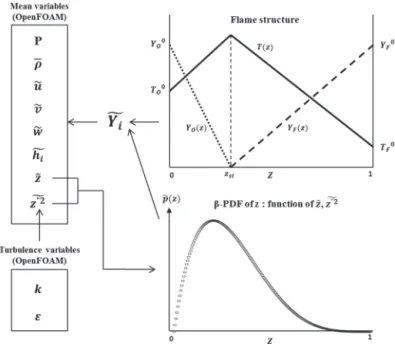
3) The steady laminar flamelet model

The Steady Laminar Flamelet Model (SLFM) represents a method available to connect the solution of the flamelet equations and the solution of the RANS equations. In this model the fluctuations of variables like temperature and species mass fraction are taken into account by incorporating a probability density function (PDF) to calculate the mean quantities. Therefore, this approach ensures that the chemistry is reduced to the transport equations for the mixture fraction and its variance that are solved in the standard CFD procedure, while species mass fractions are derived from the calculated mixture fraction fields. The reaction chemistry can be calculated using an equilibrium algorithm. In section 2.2 the mixture fraction Z gives the possibility to reduce the number of transport equations. This is consistent only if an additional assumption is made: the flame structure depends only on mixture fraction Z and on time t [6]. This assumption can be summarized as

= ( , )

= ( , ) (17)

and justified by changing the variables in the species and temperature equations from (x

, x

, x

, t) to (Z, y

, y

, t) like explained in Fig. 2.1. If the flame is thin, gradients along y

and

y

. This makes the flame structure locally one-dimensional and function of Z and t. This leads the flame front to be viewed as an ensemble of small laminar flames also called flamelets.

There are thin reactive-diffusive layers embedded within non-reacting turbulent flow field [6].

Under this assumption, the species mass fraction conservation equation can be rewritten as

= + = + 1

2 (18)

The temperature equation can be replaced as

= + 1

2 (19)

Equations are called the flamelet equations. In these equations, the scalar dissipation rate χ depends on spatial variables (x

) and controls mixing. Once χ is specified, the flamelet equations can be solved in space to provide the flame structure

III. SLFM IN OPENFOAM A. OpenFOAM

Open Field Operation and Manipulation (OpenFOAM) is an open-source Computational Fluid Dynamics (CFD) software package written in C++ language, which was first developed in the late 1980s at Imperial College, London, and was released as open source in 2004 and currently distributed by OpenFOAM foundation [7]. One of the advantages of OpenFOAM is its applicability for wide range of features such as solid dynamics, turbulent flow, reacting flow, electromagnetic field, particle dynamics and so on.

OpenFOAM has been released as free and open-source

Fig. 2. Code structure of the SLFMFoam.

Fig. 1. Overview of OpenFOAM structure [7].

program, so it can be freely customized and extended by users without any license cost. OpenFOAM was developed as an object-oriented code written C++ language, which leads the high modularity. Hence the code is easy to customize. Many solvers, libraries and utilities are already implemented in OpenFOAM. OpenFOAM also provides easy parallelization of application. Unstructured polyhedral mesh is applicable in OpenFOAM as well.

B. SLFMFoam

In this section the solver SLFMFoam is described.

SLFMFoam is an OpenFOAM application that developed to predict the non-premixed flames. In computational models based on the SLFM, the mean species mass fractions are usually pre-computed and tabulated according to the mean mixture fraction, variance of the mixture fraction and scalar dissipation rate.

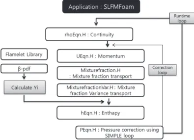
In Fig. 2 Flamelet Code computes the species mass fractions Y

(Z) by solving the flamelet equations and pre- tabulates species mass fractions in flamelet libraris. And then, The species mass fractions are passed to SLFMFoam that calculates ( ) combining Y

(Z) and the β-PDF. The continuity equation is solved in rhoEqn.H, followed by the so called SIMPLE (Semi-Implicit Method for Pressure-Linked Equations) loop. During the SIMPLE loop other equations are solved. The routine Mixturefraction.H, MixturefractionVar.H are called, solving the equations for and for

. In SLFMlookup.H the species mass fractions for each cell ( ) are computed using the interpolation of flamelet table.

The updated enthalpy field is computed in hEqn.H and used to estimate the temperature field with the mean mass fractions provided by the SLFM library. Fig. 3 shows the overall process of computation.

IV. APPLICATION TO THE HRSG

The Heat Recovery Steam Generator (HRSG) is a component used in power plants that come in different sizes with different steam production capacities. The HRSG can be either horizontally or vertically erected. The layout of the power plant is a factor when choosing the horizontal or the vertical design, but the main process remains the same. The HRSG uses the energy stored in the exhausts from a gas turbine in order to produce steam that can drive a steam turbine [8]. That is the main element that makes the concept of combined cycle possible.

A. Heat Recovery Steam Generator

The main components in a combined cycle power plants are the gas turbine, steam turbine and HRSG. The efficiency of the combined cycle power plant is influenced by the efficiency of the independent systems. The HRSG forms the heart of the combined cycle and its performance has a direct impact on the overall efficiency of the combined cycle system. Most of HRSGs are equipped with supplementary duct burners.

Supplementary firing is appropriate in the HRSG because there is enough oxygen available in the exhaust gas to cause combustion, as only a part of oxygen contained in the air is used for combustion in the gas turbine. This results in increasing the efficiency of the system by increasing steam production. A detailed illustration of the components of HRSG is shown Fig. 4.

B. Case description

The computational analysis was performed about three cases. And the detailed condition was shown to the Table 1 on the next page. The fuel is the natural gas, and the gas turbine load is divided into 100%, 60% according to the driven condition of the gas turbine. The fuel load calculated on the basis of the case C1 in which the most amount of fuel is

Fig. 3. Overall flow chart of the SLFMFoam.

Fig. 4. Illustration of the components of the HRSG.

injected.

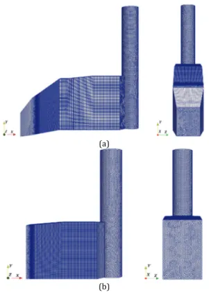
The computational mesh is generated using 3-D hexahedral, tetrahedral and hex-wedge mesh types, which provides better representation of the geometry and at the same limits the overall mesh size. To avoid excessive computational load, computational domain is divided into two stages: the first and second stages. Outflow from first stage is supplied as inlet boundary condition of the second stage. The number of element for mesh of first stage is around 7,000,000 and second stage is 9,000,000 as shown in Fig. 5.

Boundary conditions for duct burner nozzles are specified for each condition. The mass flow rate of fuel is calculated using the operation data. The geometrical area of nozzles is modeled to correctly represent the velocity and

direction of the actual fuel injection into the HRSG.

It is not practically possible to show the shape of heat exchanger so that it is replaced with the proper size of porous media region with pressure drop and heat transfer. This allows the user to input the heat sink and pressure drop characteristics separately for each of the heat exchanger. The values for heat sink and pressure drop are set using performance data.

For all of the results of HRSG discussed in this section the heat loss from the walls is assumed to be negligible. Therefore, the wall is treated as a perfectly insulated wall with no heat loss by applying the boundary condition and with no slip boundary condition.

Table 2 shows numerical method and model are used in simulation for the HRSG. The second order upwind scheme was used for the conservation equation of momentum, turbulent kinetic energy, turbulent dissipation rate, mean mixture fraction and mean mixture fraction variance. The realizable k-ε model is used based upon the results of validation in previous chapter.

C. Results and discussion

This chapter discusses the simulation results for HRSG.

Simulations are carried out for three different cases: C1, C2 and C3. All included in this Chapter are non- dimensioned result by using the specific value.

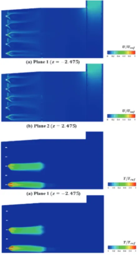
Figure 6 shows the contours of velocity and temperature distribution about x-y normal planes relating to the case C1.

Fig. 6. Velocity and temperature distributions for the case C1 in the first stage.

(a)

(b)

Fig. 5. Computational mesh for the HRSG. (a) The first stage. (b) The second stage.

Table 1

Operating conditions of the HRSG cases

C1 C2 C3

Fuel Type Natural Gas

Gas turbine load (%) 100 100 60

Fuel load (%) 100 13 53

Activated Burner (#) 15 8 12

Table 2

Numerical method and model in simulation of the HRSG Combustion model Steady Laminar Flamelet Model

Turbine model Realizable k-ε

Discretization 2nd order upwind

Mesh 7,228,341 cells (1st stage)

8,951,869 cells (2nd stage)

Since, the burners are symmetrically arranged based on the y-axis, the result about four burners is included in one plane.

The non-uniformity of flow in vicinity of the inlet is eased while it passes by the distribution plate. However, the flow in the near burner remains still non uniform. The flow distribution can be changed depending on the burner location.

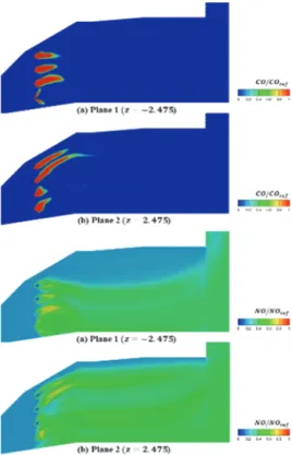
Because the lower side incoming flow is faster about 10 m/s, the burners located in the lower side get a more amount of oxidizer than the upper side. Moreover, as to the lower side, the mixing occurs actively because the recirculation zone due to swirl effect is generated in wide region. In Fig. 7, the large amount of carbon monoxide is generated in the upper side than lower side. And it is continued to near the heat exchanger region. The results of NO concentrations are similar to that of temperature fields because the production of NO is the close connection with peak temperature.

While the burnt gas in the first stage combustor passes through the heat exchanger region, the temperature descends and the flow loss the momentum. Therefore, the gas flowing into the second stage has the relatively uniform velocity distribution.

Fig. 8 show the contours of velocity and temperature distribution in the second stage. In the case C1, eight burners are operated among installed ten burners. The difference of the flow and temperature distribution for each burner is small compared with the result of the first stage. The gas flowing into second stage has low O

concentration so that it is difficult that injected fuel burns completely in the front part of the combustor.

Fig. 7. CO and NO concentrations for the case C1 in the first stage. Fig. 8. Velocity and temperature distributions for the case C1 in the second stage.

Fig. 9. Velocity and temperature distributions for the case C2 in the first stage.

The case C2 uses a little amount of fuel compared with the C1 and operates eight burners. In Fig. 9 the distribution of velocity and temperature shows the difference for each burner like the case C1. Whereas, it can confirm that CO is generated with the small quantity because there is enough amount of oxygen which can burn all the fuel in the front part of the combustor unlike the case C1. The second stage results of case C2 in Fig. 10 shows that a large recirculation zone is formed near the burners. Comparing with the result of the case C1, jet velocity and mass flow rate have the considerable influence to the formation recirculation zone, which makes the results of flames of ‘V’ shape of the Fig. 10.

In the case C3, a small amount of gas turbine exhausts enter the inlet of the HRSG unlike the previous cases. Because the composition of oxygen is high comparison with the other cases and the twelve burners are operated, the amount of oxidizer is sufficient for the complete combustion to occur.

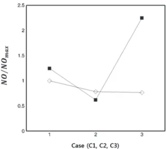
This can be proven through formation of locally high temperature zone only near the burners in Fig. 10. Therefore, the amount of CO is less than the case C1. In contrast, production of NO is increased significantly in Fig. 11, which shows the production of nitrogen monoxide is shown to be more dependent on the equivalent ratio of the local regions than the total equivalent ratio.

Comparison of predicted and measured data is shown in Table 3. All data represent the ratio of measured and predicted data at outlet of the HRSG so that the closer to one means that the difference between the measured and predicted data is less. In general, the mean temperature and concentrations of exhaust gas at outlet are reasonably

Fig. 10. Velocity and temperature distributions for the case C1 in the second stage.

Fig. 11. Velocity and temperature distributions for the case C3 in the first stage

Table 3

Comparison with results for experimental data

C1 C2 C3

Temperature 1.09 0.97 1.07

O2 Concentration 0.84 1.11 0.98

CO Concentration 0.47 0.53 1.08

Fig. 12. CO and NO concentrations for the case C3 in the first stage.

predicted for all cases. the new solver based on OpenFOAM shows excellent predictive capabilities. Overall trends are consistent between predicted and experimental data in Fig.

12.

V. CONCLUSION

The main purpose of this study is development of the Steady Laminar Flamelet Model for RANS simulation of non- premixed combustion based on OpenFOAM. The developed solver used to analyze the behavior of the HRSG in an industrial combined cycle power plant.

The steady laminar flamelet model assumes turbulent combustion composed of small laminar flamelets and turbulent effects are incorporated in the parameter called scalar dissipation rate (SDR), so that local flame structures can be described oin terms of the mixture fraction and scalar dissipation rate.

OpenFOAM, open-source CFD toolbox, is used to implement the SLFM. OpenFOAM turbulent flow solver are augmented with mixture fraction, mixture fraction variance transport equations, PDF integration and SDR calculation algorithm are implemented. For each iteration, mass fractions of chemical species are referenced from pre-tabulated flamelet library.

A HRSG is simulated with the SLFMFoam. Concerning the arrangement of burners and heat exchangers, the system is divided into two subsystems and simulations are done separately. Upstream simulation results are utilized as

boundary conditions of downstream simulation, which reduces computational requirements.

In the HRSG system, distribution plates are placed to decrease the non-uniformity of gas turbine exhaust gas that flows into HRSG. Since system’s efficiency is very sensitive to the plates, they are modeled with exact geometry without simplification. However, since the heat exchangers consist of a number of tube modules whose geometry are very complex, instead of modeling the actual geometry, the heat exchangers are modeled as porous media zones where pressure loss and heat sink occur.

Three simulations with varying fuel injections and gas turbine exhaust gas flow rates were conducted and the results were compared to measurements at the system outlet.

Predicted temperature and emissions and those from the measurements show the same trend and agreed in quantitative manner as well. Since flow patterns around the burners differ significantly, CO generation of each burner is compared to their influence. Burners around which large recirculation zone is formed produce less CO. Thus, altering burners’ orientation and fuel injection angle which affect the flow around, may improve the emission characteristics.

In this study Steady laminar flamelet model (SLFM) solver is implemented in OpenFOAM and the solver is used for simulation of the HRSG system. Flow and combustion characteristics of the system under operating conditions are analyzed to derive performance improvement, which will be used to reduce time and costs required for the optimum design.

REFERENCES

[1] Vytla, V.S., “CFD Modeling of Heat Recovery Steam Generator and its components Using Fluent,” Master’s Thesis, Univ. Kentucky, USA, 2005.

[2] Ivan, F., Galindo, G., Ana, K., “CFD Simulations of Heat Recovery Steam Generators Including Tube Banks,” ASME Conference, 2014.

[3] Magnussen, B.F., Hjertager, B.H., “On Mathematcal Modeling of Turbulent Combustion with Special Emphasis on Soot Formation and Combustion,” 16th Symp. on Combustion, 1976, pp.719-729.

[4] Coelho, P.J., Peters, N., “Unsteady modelling of a piloted methane/air jet flame based on the Eulerian particle flamelet model,” Combust. Flame Vol. 124, Issue 3, 2001, pp. 444~465.

[5] Poinsot, T., Veynante, D., Theoretical and numerical combustion, R.T.

Edwards, Inc., 2005.

[6] Peters, N., “Laminar diffusion flamelet models in non-premixed turbulent combustion,” Progress Energy Combustion Science, Vol.10, Issue 3, 1984, pp.319 ~339.

[7] Openfoam user guide, 2.3.0, OpenFOAM Foundation, 2013.

[8] Horkeby, K., “Simulation of Heat Recovery Steam Generator in a Combined Cycle Power Plant,” Institutionen för systemteknik Department of Electrical Engineering.

[9] Vytla, V.S., “CFD Modeling of Heat Recovery Steam Generator and its components Using Fluent,” Master’s Thesis, Univ. Kentucky, USA, 2005.

Fig. 13. Comparison with results for experimental data at different cases.

(square: predicted data, diamond: experimental data)