Initial Mass Function and Star Formation History in the Small Magellanic Cloud
Ki-Won Lee*
Institute of Liberal Education, Catholic University of Daegu, Gyeongsan 712-702, Korea
Abstract: This study investigated the initial mass function (IMF) and star formation history of high-mass stars in the Small Magellanic Cloud (SMC) using a population synthesis technique. We used the photometric survey catalog of Lee (2013) as the observable quantities and compare them with those of synthetic populations based on Bayesian inference.
For the IMF slope (Γ ) range of −1.1 to −3.5 with steps of 0.1, five types of star formation models were tested: 1) continuous; 2) single burst at 10 Myr; 3) single burst at 60 Myr; 4) double bursts at those epochs; and 5) a complex hybrid model. In this study, a total of 125 models were tested. Based on the model calculations, it was found that the continuous model could simulate the high-mass stars of the SMC and that its IMF slope was −1.6 which is slightly steeper than Salpeter's IMF, i.e., Γ = −1.35.
Keywords: initial mass function, star formation, Magellanic Cloud, Bayesian inference
Introduction
The main property that determines the fate of a star is its initial mass, although other factors (such as metallicity, mass-loss rate, rotation, and magnetic field strength) also play a role in its evolution (Maeder and Meynet, 2003, 2004). Once the mass of a star is known, we can, in principle, estimate such quantities as luminosity, radius, and effective temperature at any phase of stellar evolution. Furthermore, we can understand the evolution of a galaxy which is composed of stars of various masses. The accurate determination of the initial mass function (hereafter, IMF) and its variation in space and time provides fundamental constraints on star formation in the Galaxy and external galaxies in terms of their dynamical and chemical evolution.
In a seminal work, Salpeter (1955) investigated the IMF of stars in the solar neighborhood and found that the IMF slope (Γ ) is −1.35 which is now referred to
as a “Salpeter slope”. Miller and Scalo (1979) examined both observational and theoretical evidence relating to the IMF and star formation history in the solar neighborhood. Later, Scalo (1986) produced a thorough review of the subject and highlighted the remaining problems for IMF studies over a wide range of systems (e.g., field stars, star clusters, and nearby galaxies). Gilmore and Howell (1998) later presented new results for the stellar initial mass function. Overall, it seems that there is no strong evidence for IMF variations; most results follow the Salpeter slope within observational errors, regardless of mass ranges and/or targets, i.e., they confirm the
“universal IMF”, although there are some suggestions for a steeper IMF slope for the massive stars (Massey et al., 1995; Lamb et al., 2013). A universal IMF is often considered to imply a universal star formation process.
The IMF is one of very important physical quantities in astronomy because its accurate determination is crucial to fundamental astrophysical problems: the formation and evolution of star clusters, star formation history in the Galaxy and external galaxies, dynamical and chemical evolution of galaxies, dark matter problem, and so on. As regards the IMF study of the SMC, Humphreys (1983) studied the luminous-star population in the very metal-poor galaxy and showed
*Corresponding author: [email protected]
*Tel: +82-53-850-2573
*Fax: +82-53-850-3800
This is an Open-Access article distributed under the terms of the Creative Commons Attribution Non-Commercial License (http://
creativecommons.org/licenses/by-nc/3.0) which permits unrestricted non-commercial use, distribution, and reproduction in any medium, provided the original work is properly cited.
a steeper function for the highest masses. Hill et al.
(1994) found an average slope of Γ = −2.0±0.5 for M
>9 M⊙ from 14 associations in the Magellanic Clouds.
Massey et al. (1995) also investigated the massive star populations of the SMC and reported that the slope of the IMF is very steep, Γ = −3.7±0.5 for field-stars.
More recent results on the IMF of the SMC are found in the review of Bastian et al. (2010).
It has been acknowledged that population synthesis methods are a powerful tool for the study of stellar systems, clusters, or galaxies in association with stellar evolutionary models (e.g., Schlesinger, 1969; Schild and Maeder 1983; Greggio, 1986; Tosi et al., 1991;
Tolstoy and Saha, 1996). In particular, Leitherer (1998) compared the observational color-magnitude diagram (CMD) of a cluster with that of models from stellar atmospheres and evolutionary tracks, which allows one to constrain the IMF and star formation history of its parent galaxy.
In this study, we investigated the IMF and star formation history of high-mass stars in the Small Magellanic Cloud (SMC) by employing a stellar population synthesis technique. Unlike previous studies, we transformed the theoretical quantities of synthetic population stars into the observable ones. As observational quantities, we used the photometric survey catalog of Lee (2013) (hereafter, paper I). The present paper is organized as follows. We briefly describe the population synthesis method in Section 2 and introduce Bayesian statistics used for comparing the observational quantities with synthetic ones in Section 3. We present results regarding the star formation histories and IMF slopes in Section 4.
Finally, the major findings of this study are summarized in Section 5.
Population Synthesis Method
Stellar evolution model
The most widely used stellar evolutionary models are from the Geneva and Padova groups. Both types of models can be used to calculate evolutionary tracks for various metal abundances (Zs) and masses. However,
we use the Geneva models in our population synthesis code because they were calculated for a Z=0.004 grid (Charbonnel et al., 1993), i.e., the metal abundance of the SMC (Lequeux et al., 1979). Recently, Maeder and Meynet (2001) found that the effect of rotation caused the evolutionary tracks to move toward lower effective temperatures, extending the main sequence bandwidth, and that the use of non-rotating tracks would cause the mass to be overestimated at lower metallicity. However, the evolutionary model incorporating rotational effects is not considered here, because the main purpose of this study is to compare with the results of previous studies, for the most part, based on the non-rotating evolutionary model. Most of all, it is practically impossible to simultaneously consider all the individual speeds.
Initial Mass Function
The IMF, φ (m), is defined as the fraction or number of stars formed per unit mass interval, dm, at birth. In practical applications, the most commonly adopted form is the power law distribution:
φ (m)=φ0mγ, (1)
where φ0 is a constant. It is convenient, in practice, to replace the IMF φ (m) by ξ (logm), which gives the fraction or number of stars formed per unit logarithmic (base ten) mass interval at birth (e.g., Salpeter, 1955). The relation between the two functions is:
ξ (logm)=ξ0mγ +1=ξ0mΓ, (2) where ξ0=φ0ln(10) and Γ =γ +1. In this equation, the slope found by Salpeter is Γ = −1.35 or γ = −2.35.
On the basis of Equation (1), the number of stars between masses m and m +dm, dN, is given by:
dN(m)=φ (m)dm=φ0mγdm. (3)
Because Equation (3) has an analytical integral solution, we can use the inversion method in a Monte Carlo simulation (Press et al., 1992) to generate a synthetic population. For a given minimum and maximum mass interval, we synthesized the populations
with various IMF slopes, i.e., Γ = −1.1 to −3.5 with steps of 0.1.
According to the evolutionary models, a 3 M⊙ star corresponds to B ~19.0, which is the lower magnitude limit of the photometric sample in paper I. However, we choose 2 M⊙ as a safe minimum mass value. The selection of maximum mass is somewhat arbitrary. We choose 120M⊙, the highest mass for which evolutionary tracks are available, as the maximum mass, although Crowther et al. (2010, and reference therein) suggested ~300 M⊙ as the upper mass limit for massive stars. Regarding the number of stars within a synthetic population, NSP, we included 100 times more stars than that of our photometric subsample, NPS, (i.e., NSP=100×NPS) in order to improve the statistical analysis.
Star formation history
Gardiner and Hatzidimitriou (1992) studied stellar populations in the SMC and found that the star formation rate in the SMC has decreased over the past 2 Gyr, excluding the active star formation regions in the core and in the wing. As far as the chemical evolution is concerned, there also have been many studies of the star formation history in the SMC. Most of these studies agreed that the SMC has markedly different features compared to those of our Galaxy in terms of the metallicity (Lequeux et al., 1979), age distribution of star clusters (Olszewski et al., 1996;
Westerlund, 1997), element ratios (Pagel and Tautbvaišienè, 1998), and so forth (see van den Bergh, 2000 for comprehensive review).
Harris and Zaritsky (2004) investigated the star formation and chemical enrichment history of the SMC using their photometric survey (Zaritsky et al., 2002). Although there are systematic differences of ~2 Gyr, their results showed good overall agreement with the burst model of Pagel and Tautbvaišienè (1998).
Harris and Zaritsky (2004) divided the SMC star formation history into three epochs: 1) an early epoch (t >8.4 Gyr), in which about 50% of the SMC stars were formed; 2) an intermediate epoch (3<t <8.4
Gyr), in which the SMC has a long quiescent period;
and 3) an active epoch (t <3 Gyr), in which there has been active star formation caused by bursts at 2.5 Gyr, 400 Myr, and 60 Myr. However, according to the Geneva evolutionary model, stars more massive than only ~6 M⊙ left the main sequence stage after 400 Myr. Therefore, epochs older than 400 Myr are inappropriate considering the minimum mass in this study. For the reason, we choose 60 Myr as the burst epoch. In addition, we choose an arbitrary epoch, 10 Myr, to test the starburst history of high-mass stars of the SMC.
In this study, we assumed five types of star formation models: 1) continuous; 2) burst with single bursts at 10 and 3) 60 Myr and 4) double bursts at both epochs; and 5) a more complex hybrid model.
• Continuous star formation model. Although it is known that the oldest cluster in the SMC is 12 Gyr old (Stryker et al., 1985), the lifetime of a 2 M⊙ star is only 1.08 Gyr, according to the Geneva evolutionary library for Z =0.004. So we used 2 Gyr, which is sufficiently longer than the lifetime of our minimum mass star, as the input for age. One of the validations of this model is given by the smooth star formation theory of Pagel and Tautbvaišienè (1998), which can be approximated as continuous models for the last 2 Gyr.
• Burst star formation models. To simulate a starburst history, we assumed single bursts at 10 Myr and 60 Myr epochs. With equal contributions from each single burst, we also test a double burst model.
So the burst models are subdivided into three models:
two single and one double burst models.
• Complex star formation model. To consider the complex star formation history in the SMC, we also test a single “complex” model with contributions of 50, 25, and 25% of the numbers from the continuous and the bursts models at 10 and 60 Myr, respectively.
We considered a total of 125 population models in our study − five types of the star formation models for twenty five different IMF slopes− and compared each with three independent photometric subsamples.
Selection effects
Before comparing the photometric samples with synthesized populations, we have to consider the selection effects and incompleteness in our observations.
One of the advantages of transforming theoretical data into observable parameters (i.e., method used in this study) is that the corrections are more easily, accurately, and transparently applied to the reverse process.
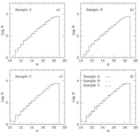
In practice, it is impossible to simultaneously compare all the photometric survey data of paper I, which comprises 1.3 million stars, with a synthesized population. Therefore, we randomly collected subsamples containing about 5% of the stars with B <19.0 and (B- V)<0.6, which amounts to ~23,000 stars. Although we found that the number distribution of the 5% of stars represented that of the whole photometric survey well (see Fig. 6 in paper I), we extracted three observational subsamples to reduce the possibility that
the subsamples are biased. Fig. 1 represents the number distribution of the three subsamples, labeled as A, B, and C. In the first three pictures, the solid lines are the actual number distributions of subsamples, the dotted lines are the totals of our selected photometric data. The last picture is plotted in order to compare together the number distibution of each subsample. As can be seen in Fig. 1, the distributions show good agreement with total distribution except for the stars brighter than 13 magnitude, which are caused by the scarcity of brighter stars.
Suppose that P(Bi), P(Vi), and P(Ri) represent the detection probabilities of the ith artificial star in B, V, and R bands, respectively, which are given by the photometric completeness of our observations in each band (see Table 2 of paper I). We then define the possibility that the synthetic star will be selected, PS, for two extreme cases:
Fig. 1. The number distribution of three observational subsamples used for comparison with the models. In Figures a), b), and c), the solid lines are the number distribution of subsamples, the dotted lines are that of our selected photometric data normal- ized to each subsample. Figure d) shows the comparison of each subsample.
1) If a field is sparse, i.e., limited by magnitude, then we considered that the probability in each filter is independent such that PS is the product of the probability in each filter (i.e., PS=P(Bi)×P(Vi)×P(Ri)).
2) If a field is dense, i.e., limited by crowding, the photometric completeness shows a similar feature regardless of filter, i.e., P(Bi)~P(Vi)~P(Ri). In this case, the detection of a star depends mainly on position, rather than on magnitude. This means that P(Bi), P(Vi), and P(Ri) are not independent; therefore, we choose PS as the minimum probability (i.e., PS= min[P(Bi), P(Vi), P(Ri)]).
In Fig. 2, we present the relative photometric completeness, normalized to 1, to show that this approach is reasonable in practical terms. Lastly, we do not need to correct for the effect of incompleteness in each survey area, because the important factor in the comparison is not the absolute number of stars but the relative numbers (per unit interval in color and magnitude).
Transformation into observable parameters Theoretical stellar evolutionary model calculations for a given age and mass are (interpolated) current mass, luminosity (L), and effective temperature. We then transform those parameters into color indices calculated by Bessell et al. (1998) in order to compare them with our photometric data.
Bessell et al. (1998) studied wide band colors, bolometric corrections, and temperature calibrations for O-M stars using various model atmospheres (references therein). According to their results, most colors show good agreement with empirical relations, except the (B-V) color for K giants, M dwarfs, and M giants. In this study, we adopt their grid and note that the minor disagreement in (B-V) for cool stars has minimal influence on our study, which deals mostly with high-mass stars.
We first interpolated grids given by Bessell et al.
(1998) using the effective temperature and the surface gravity from the outputs of theoretical stellar evolutionary Fig. 2. The relative photometric completeness as a function of magnitude in the dense (upper panel) and in the sparse region (bottom panel). The values are normalized to 1.
models, and then transformed them into synthetic color indices, (B-V) and (V-R), using color excesses of E(B-V)=0.107 and E(V-R)=0.094*, and the ratio of selective extinction to redding of RV=3.1 (e.g., Schultz and Wiemer, 1975). For the model apparent V magnitude, we used the following relation.
V =Mbol,⊙−2.5log(L/L⊙)−B.C.+D.M.+AV, (4) where Mbol,⊙ is the bolometric magnitude of the sun, and D.M. is the distance modulus and AV is the interstellar extinction in V magnitude of the SMC. We used the values of Mbol,⊙=4.47 (Bessell et al., 1988), D.M.=18.89 (Harries et al., 2003), and AV=0.267 (paper I). Because Bessell et al. (1998) only constructed grids for the range from 3,500 to 50,000K in effective temperature, we extended their bolometric corrections (B.C.) using the relation of Howarth and Prinja (1989) for temperatures above 50,000K, which is known to give good accuracy.
For details of the population synthesis method used in this study, refer to the work of Lee (2005).
Bayesian Statistics
To obtain a quantitative comparison of our photometric subsamples with models, we employed the statistical analysis developed by Tolstoy and Saha (1996). They adopted Bayesian inference to estimate the likelihood between the model magnitude-magnitude diagram (MMD) and observational MMD, but their analysis is easily generalized to other parameter spaces (e.g., CMD).
Bayesian inference
Bayesian inference is one of the best methods to determine the model giving the best representation (relative probability or likelihood) of the observation.
Suppose that the probabilities of events A and B are P(A) and P(B), then the probability that A and B will
happen, P(A,B), is:
P(A,B)=P(A)P(B|A)=P(B)P(A|B), (5) where, P(B|A) is the probability of B given A, and P(A|B) is the probability of A given B. From equation (5),
P(B|A)= , (6)
which is conventionally known as Bayes’ theorem. As for other probabilities, P(B|A) have to normalized, so Bayes’ theorem (Equation 6) is
P(B|A)= , (7)
where .
Now consider an observed data set composed of n points, D =(D1, ···, Dn), and the models describing the data set, M =(M1, ···, Mi, ···). From Bayes’ theorem, the probability of a model Mi given the observed data set D, P(Mi|D), is:
P(Mi|D)= . (8)
In practical cases as well as in observational data, the probability is not continuous but discrete. Therefore, the normalization can be replaced by the summation.
i.e.,
. (9)
However, because it is impossible to consider every possible model, i.e., , Bayes’ theorem is rewritten as a relative possibility, or as the proportional relation:
P(Mi|D) ∝ P(Mi)P(D|Mi). (10) P B( )P A B( )
P A( ) ---
P B( )P A B( ) P B( )P A B( ) Bd
∫
--- P A( )=∫
P B( )P A B( ) BdP M( )P D Mi ( i) P D( ) ---
P D( ) P M( )P D Mi ( i)
∑
i=
P M( )i i
∑
∞* At the time of model calculations, we had obtained different values for the distance modus and color excesses to the final values presented in paper I. Because the values used in model calculations are only slightly different, and because the model calculations require large amounts of computer time, we did not re-calculate using new values. However, we believe that this has negligibly affect on our results.
Likelihood method
Again, suppose that there is an observational data set D consisting of N pairs of points in two-dimensional coordinates, X=X(x, y), with uncertainties σ :
D = D(Dx(n), Dy(n))
σ = σ (σx(n), σy(n)), n =1, ···, N. (11) In addition, suppose that there is a model M consisting I pairs of points in the same dimensions,
M = M(Mx(i), My(i)), i =1, ···, I. (12) In our case, the x-dimension is the color index and y is the magnitude on a CMD plane.
Assumed a Gaussian distribution in its positional uncertainty, the (unnormalized) probability which a data point is matched to the entire ensemble of model points, Sn(D), is
Sn(D)=
. (13)
The natural logarithm of the likelihood, lnL, is the Nth product of the probabilities of each point for all data points, i.e.,
lnL=ln . (14)
As emphasized by Tolstoy and Saha (1996), the likelihood is only a relative probability; therefore, they defined a “perfect” likelihood (lnLd) from the model using the data points themselves. It is used as the zero point for each model, such as ln(Lj/Ld), which is the relative likelihood for the jth model.
Results
Continuous model
First, we considered a continuous star formation model for the SMC. In the Geneva evolutionary models, the maximum age for a 2 M⊙ star with Z=
0.004 is 1.08 Gyr. Hence, in this model, we assume that stars were continuously formed from 2 Gyr ago.
Although the smooth model of Pagel and Tautbvaišienè (1998) for the star formation history in the SMC shows a small continuous decrease within recent 2 Gyr (see their Fig. 2), it can be approximated as a constant continuous model, providing a theoretical base for the validity of this model.
With model sets containing one hundred times the population of observed stars for a randomly selected 5% sample (i.e., 2,300,000 synthetic stars) and with IMF slopes varying from –1.1 to –3.5, we calculated maximum likelihood values and present the results in Fig. 3. The upper panel shows the likelihood for the (B-V) versus V plane, and the lower panel shows (V- R) versus V for the three samples (A, B, and C), which are indicated with different lines. For the comparison, the samples B and C are normalize to the sample A by adding the values presented in each panel.
In general, they show a very similar pattern for all three samples for a given coordinate set: a slow increase up to Γ = −1.6 in the (B-V) coordinate and a rather steep decrease after Γ = −2.1, while continuously decreasing in the (V-R) coordinate. In the comparison between coordinates, the values in (B-V) vs V are 1.5 times larger than those in (V-R) vs V. The maximum variation amongst the sample sets is ~5.7% in (B-V) vs V (e.g., ~ −1.476×10⁵ in sample A and ~−1.560×
105 in sample B at Γ = −1.6). This difference is smaller than in (V-R) vs V, ~0.45%. Therefore, we can know that there are no significant differences amongst three subsample. Another fact is that the sample showing high values in one color index does not have the same result in the other. For example, on average, sample B has the lowest values in (B-V) vs V coordinate; however, sample C shows the lowest in (V-R) vs V.
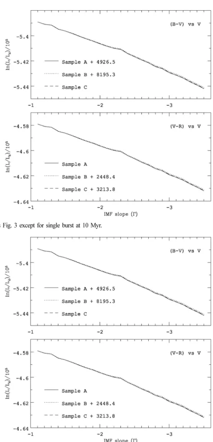
Single burst models
In this model, we investigated burst star formation history at two different epochs; a burst at 10 and one at 60 Myr. The results are presented in Figs. 4 and 5 for the bursts at t =10 and 60 Myr, respectively. All notations are the same as in Fig. 3. On the whole, the 1
---I 1 2πσx( )σn y( )n ---
exp
i 1=
∑
I –(---M i() D n2σ n–( )( )2 )2×
Πn 1N= Sn( )D
[ ]
burst model at 10 Myr shows smooth variations compared to other models and maxima at Γ = −1.3, the slope of the Salpeter IMF, in both coordinates.
The fact that the single burst model at a relevant epoch yields a maximum value at the traditional IMF slope is interesting because the targets of most IMF studies on the IMF are for the clusters/associations, which are assumed to have the same ages, and most of them show the universal IMF slope of Γ = −1.3. On the other hand, the burst model at 60 Myr represents a continuous decrease as the IMF becomes steeper;
therefore, it does not have a maximum within our IMF slope ranges. This is a natural consequence because, as previously mentioned, the lifetime of stars more massive than ~6 M⊙ is shorter than 60 Myr (according to the Geneva evolutionary model), while our catalog stars are mostly massive. Even if we perform the model calculations for the extended IMF ranges, the maximum value seems to not approach that of the continuous model.
Considering the fact that the SMC is a galaxy consisting of stars of different ages and that high-mass stars were formed quite recently in comparison, the poor results for the burst models are not unexpected, especially for a burst at an old epoch.
Double bursts models
We considered two starburst events taken place at different epoch in another model, with equal proportions from each single burst, i.e., 50% at 10 and 60 Myr.
An interesting result is that it shows, on average, higher maximum likelihood values than those of for each individual burst, although this model still yields lower values than the continuous one (see Fig. 6). For the reason mentioned above, the double burst model is more realistic than a single burst model for the SMC, a galaxy composed of stars formed in different eras.
In general, this model follows the tendency of the burst model at 60 Myr, and has slightly higher values than those of the single models in the maximum Fig. 3. Likelihood results for the continuous model. The upper panel is result from (B-V) versus V and the lower is from (V-R) versus V for the three different sample sets.
Fig. 4. The same as Fig. 3 except for single burst at 10 Myr.
Fig. 5. The same as Fig. 3 except for single burst at 60 Myr.
likelihood statistic calculations. The likelihood values in the (V-R) vs V coordinate are higher than in the (B-V) vs V coordinate (reflecting differences in the photometric errors), like other burst models.
Complex models
Lastly, we tested a complex model based on the previous model data sets: consisting of 50, 25, and 25% contributions from the continuous and burst models at 10 and 60 Myr, respectively, and present the results of the complex model in Fig. 7. The impressive features of this model are that all our complex models show only slightly lower likelihood values compared to the continuous model and have a steep IMF. A peak of the three samples in the (B-V) vs V plane occurs at Γ = −2.5, with −1.6, the same value as for the continuous model, in the (V-R) vs V plane. The feature which one should bear in mind with this model is the possibility that the more delicate complex model can produce better results
than the continuous model. Of course, it is true that any arbitrary well-tuned complex model can give better results. In any case, the differences between this and the continuous model in the peak value are quite small; for example, only ~4.5% variation at Γ = −1.6 in (B-V) vs V plane.
Summary
We studied the IMF and star formation history of massive stars in the SMC using a population synthesis method containing two libraries: an evolutionary model from the Geneva group and a transformation grid, the result of stellar atmosphere models, from Bessell et al. (1998). In selecting our subsamples and models, we constrained the stars to be B <19.0 and (B-V)<0.6. For the photometric incompleteness according to regions, we used the results of the artificial star test technique from paper I. In contrast to other studies, we transformed the model quantities into observable Fig. 6. The same as Fig. 3 except for bursts at 10 and at 60 Myr with half of the synthetic sample from both.
ones. We then compared both on the basis of a Bayesian statistical study with various star formation histories and IMF slopes.
We used five models: 1) continuous star formation from 2 Gyr before the present; 2) single burst star formation at 10 and 3) at 60 Myr epochs; 4) double bursts at both epochs with the same contribution in number; and 5) a complex model with 50, 25, and 25% contributions from continuous and burst models in the two epochs, with the IMF slopes ranging from
−1.1 to −3.5. We performed model calculations for three randomly selected subsamples for a safe estimation.
In the following, we summarize the main results from the study of model calculations.
• The maximum likelihood values in (V-R) vs V coordinate is larger than those in (B-V) vs V in all burst models; however, the reverse is the case in the other models.
• The continuous model gives the best likelihood statistic. From this model, the slope of the IMF in the SMC is −1.6, which is slightly steeper than Salpter’s IMF slope of −1.3.
• A single burst model at the 10 Myr epoch yields the Salpeter’s IMF slope, Γ = −1.3, with lower likelihood values than those for the continuous model. The burst model at 60 Myr shows a continuous decrease as the IMF slope becomes steeper. Overall, single burst models offer the least likely result with the lowest likelihood among all the considered models. The double burst model, equally drawn from 10 and 60 Myr bursts, has higher likelihood statistic values than for a single burst.
• The complex model yields a somewhat steeper IMF slope, Γ = −2.5 in (B-V) vs V coordinate. In general, the values of maximum likelihood in this model are similar to those for the continuous one but with steeper IMFs.
Fig. 7. Likelihood results for the complex model composed of 50, 25, and 25% contributions from the continuous model and burst models at 10 and 60 Myr, respectively.
In conclusion, we suggest that the continuous star formation history, consistent with Pagel and Tautbvaišienè (1998), is the best model for representing the SMC and that the IMF of high-mass stars in the SMC is −1.6, which is slightly steeper than Salpeter’s IMF. This fact implies that the fraction of low mass stars is larger than that of high-mass ones at birth compared to in the solar neighborhood.
Acknowledgment
This work was supported by research grants from the Catholic University of Daegu in 2014.
References
Bastian, N., Covey, K.R., and Meyer, M.R., 2010, A universal stellar initial mass function? a critical look at variations, 48, 339-389.
Bessell, M.S., Castelli, F., and Plez, B., 1998, Model atmospheres broad-band colors, bolometric corrections and temperature calibrations for O-M stars. Astronomy and Astrophysics, 333, 231-250.
Charbonnel, C., Meynet, G., Maeder, A., Schaller, G., and Schaerer, D., 1993, Grids of stellar models. III. From 0.8 to 120M⊙ at Z=0.004. Astronomy and Astrophysics Supplement, 101, 415-419.
Crowther, P.A., Schnurr, O., Hirschi, R., Yusof, N., Parker, R.J., Goodwin, S.P., and Kassim, H.A., 2010, The R136 star cluster hosts several stars whose individual masses greatly exceed the accepted 150M⊙ stellar mass limit.
Monthly Notices of the Royal Astronomical Society, 408, 731-751.
Gardiner, L.T. and Hatzidimitriou, D., 1992, Stellar populations and the large-scale structure of the Small Magellanic Cloud-IV. Age distribution studies of the outer regions. Monthly Notices of the Royal Astronomical Society, 257, 195-224.
Gilmore, G. and Howell, D., 1998, The stellar initial mass function: 38th Herstmonceux conference. Astronomical Society of the Pacific Conference Series, 142, 240 p.
Greggio, L., 1986, The brightest stars in galaxies - a theoretical simulation. Astronomy and Astrophysics, 160, 111-115.
Harries, T.J., Hilditch, R.W., and Howarth, I.D., 2003, Ten eclipsing binaries in the Small Magellanic Cloud:
Fundamental parameters and Cloud distance. Monthly Notices of the Royal Astronomical Society, 339, 157- 172.
Harris, J. and Zaritsky, D., 2004, The star formation history of the Small Magellanic Cloud. The Astronomical Journal, 127, 1531-1544.
Howarth, I.D. and Prinja, R.K., 1989, The stellar winds of 203 Galactic O stars: A quantitative ultraviolet survey.
The Astrophysical Journal Supplement, 69, 527-592.
Humphreys, R.M., 1983, Studies of luminous stars in nearby galaxies. III. The Small Magellanic Cloud. The Astrophysical Journal, 265, 176-193
Lamb, J.B., Oey, M.S., Graus, A.S., Adams, F.C., and Segura-Cox, D.M., 2013, The initial mass function of field OB stars in the Small Magellanic Cloud. The Astrophysical Journal, 763, 101-114.
Lee, K.W., 2005, A photometric survey of the Small Magellanic Cloud. Ph.D. dissertation, University College London, London, UK, 222 p.
Lee, K.W., 2013, A BVR photometric survey of the Small Magellanic Cloud with a mosaic CCD. Journal of the Korean Earth Science Society, 5, 415-427.
Leitherer, C., 1998, Populations of massive stars and the interstellar medium. In Aparicio, A., Herrero, A., and Sanchez, F. (eds.), Stellar astrophysics for the local group: VIII Canary Islands winter school astrophysics.
Cambridge University Press, Cambridge, UK, 527-606.
Lequeux, J., Peimbert, M., Rayo, J.F., Serrano, A., and Torres-Peimbert, S., 1979, Chemical composition and evolution of irregular and blue compact galaxies.
Astronomy and Astrophysics, 80, 155-166.
Maeder, A. and Meynet, G., 2001, Stellar evolution with rotation. VII. Low metallicity models and the blue to red supergiant ratio in the SMC. Astronomy and Astrophysics, 373, 555-571.
Maeder, A. and Meynet, G., 2003, Stellar evolution with rotation and magnetic fields. I. The relative importance of rotational and magnetic effects. Astronomy and Astrophysics, 411, 543-552.
Maeder, A. and Meynet, G., 2004, Stellar evolution with rotation and magnetic fields. II. General equations for the transport by Tayler-Spruit dynamo. Astronomy and Astrophysics, 422, 225-237.
Massey, P., Lang, C.C., Degioia-Eastwood, K., and Garmany, C.D., 1995, Massive stars in the field and associations of the Magellanic Clouds: The upper mass limit, the initial mass function, and a critical test of main-sequence stellar evolutionary theory. The Astrophysical Journal, 438, 188-217.
Miller, G.E. and Scalo, J.M., 1979, The initial mass function and stellar birthrate in the solar neighborhood.
The Astrophysical Journal Supplement, 41, 513-547.
Olszewski, E.W., Suntzeff, N.B., and Mateo, M., 1996, Old and intermediate-age stellar populations in the Magellanic Cloud. Annual Review of Astronomy and Astrophysics, 34, 511-550.
Pagel, B.E.J. and Tautbvaišienè G., 1998, Chemical evolution of the Magellanic Clouds: Analytical models.
Monthly Notices of the Royal Astronomical Society, 299, 535-544.
Press, W.H., Flannery, B.P., Teukolsky, S.A., and Vetterling, W.T., 1992, Numerical recipes in Fortran. Cambridge University Press, Cambridge, UK, 277-280.
Salpeter, E.E., 1955, The luminosity function and stellar evolution. The Astrophysical Journal, 121, 161-167.
Scalo, J.M., 1986, The stellar initial mass function.
Fundamentals of Cosmic Physics, 11, 1-278
Schild, H. and Maeder, A., 1983, The relation between luminosity of the brightest blue star and the luminosity of its parent galaxy. Astronomy and Astrophysics, 127, 238-240.
Schlesinger, B.M., 1969, Theoretically predicted color- magnitude diagrams for clusters and the observations.
The Astrophysical Journal, 157, 533-544.
Schultz, G.V. and Wiemer, W., 1975, Interstellar reddening and IR-excess of O and B stars. Astronomy and
Astrophysics, 43, 133-139.
Stryker, L.L., Da Costa, G.S., and Mould, J.R., 1985, The main-sequence turnoff of the old SMC globular cluster NGC 121. The Astrophysical Journal, 298, 544-559.
Tolstoy, E. and Saha, A., 1996, The interpretation of color- magnitude diagrams through numerical simulation and Bayesian inference. The Astrophysical Journal, 462, 672-683.
Tosi, M., Greggio, L., Marconi, G., and Focardi, P., 1991, Star formation in dwarf irregular galaxies-Sextans B.
The Astronomical Journal, 102, 951-974.
Westerlund, B.E., 1997, The Magellanic Clouds. Cambridge University Press, Cambridge, UK, 292 p.
van den Bergh, S., 2000, The galaxies of the local group.
Cambridge University Press, Cambridge, UK, 348 p.
Zaritsky, D., Harries, J., Thompson, I.B., Grebel, E.K., and Massey, P., 2002, The Magellanic Clouds photometric survey: The Small Magellanic Cloud stellar catalog and extinction map. The Astronomical Journal, 123, 855- 872.
Manuscript received: July 31, 2014 Revised manuscript received: August 27, 2014 Manuscript accepted: September 17, 2014