JPNT 3(3), 123-129 (2014)
http://dx.doi.org/10.11003/JPNT.2014.3.3.123 J PNT
Journal of Positioning,Navigation, and Timing
1. INTRODUCTION
The Global Positioning System (GPS) real-time kinematic (RTK) is one of the methods that precisely determine the position of a user. The GPS RTK method accurately estimates the position of a user using the observables received at a GPS reference station whose position is accurately known and GPS measurements received by the user, in a relative manner. In general, a relative positioning method determines the position of a user after eliminating common errors through a double difference of the observation data of both a reference station and a user. The position accuracy of a user is affected by the ionosphere and the troposphere (Rocken et al. 1995, Wielgosz et al. 2005). If a baseline between a reference station and a user is less than 10 km, the ionospheric and tropospheric delay errors can be eliminated using a double difference technique assuming that GPS signals have passed through the similar path. In contrast, if a baseline is more than 10 km, the effects of the
Long Baseline GPS RTK with Estimating Tropospheric Delays
Byung-Kyu Choi
1†, Kyoung-Min Roh
1, Sang Jeong Lee
21
Space Science Division, Korea Astronomy and Space Science Institute, Daejeon 305-348, Korea
2
Department of Electronics Engineering, Chungnam National University, Daejeon 305-764, Korea
ABSTRACT
The real-time kinematic (RTK) is one of precise positioning methods using Global Positioning System (GPS) data. In the long baseline GPS RTK, the ionospheric and tropospheric delays are critical factors for the positioning accuracy. In this paper we present RTK algorithms for long baselines more than 100 km with estimating tropospheric delays. The state vector is estimated by the extended Kalman filter. We show the experimental results of GPS RTK for various baselines (162.10, 393.37, 582.29, and 1283.57 km) by using the Korea Astronomy and Space Science Institute GPS data and one International GNSS Service (IGS) reference station located in Japan. As a result, we present that long baseline GPS RTK can provide the accurate positioning for users less than few centimeters.
Keywords: GPS, RTK, long baseline, tropospheric delays
ionosphere and the troposphere should be considered;
and the effect of the atmosphere increases as a baseline increases (Saastamoinen 1972). In particular, in the case of long baseline RTK positioning with a baseline of more than 100 km, the effects of different crustal movements and the satellite orbit errors need to be also considered in addition to an influence of the atmosphere (Geng et al. 2011).
To precisely determine the position of a user based on the GPS RTK technique (i.e. relative positioning), GPS measurements from at least one reference station whose position is accurately known are required. In general, if a baseline is less than 10 km, the position of a user receiving a single frequency can be determined based on the RTK technique with a 1 cm-level accuracy (Fotopoulos & Cannon 2001). However, for long baselines, the determination of carrier phase integer ambiguities is difficult due to various error factors, and initial convergence time is also long (Teunissen 1995, Lawrence et al. 2006). When the baseline increases, single frequency users cannot completely correct the error from the atmosphere, compared to dual frequency users. Thus, single frequency users have the disadvantage of reduced position accuracy (Davis et al. 1985, Blewitt, 1989, Brunner & Welsch 1993). In contrast, dual frequency users can basically eliminate the effect of the ionosphere, which is the largest error factor for long baseline relative positioning, Received April 27, 2014 Revised July 10, 2014 Accepted July 11, 2014
†
Corresponding Author E-mail: [email protected]
Tel: +82-42-865-3237 Fax: +82-42-861-5610
124 JPNT 3(3), 123-129 (2014)
through the linear combination of the frequencies of two GPS signals.
The network RTK technique, which is operated based on many GPS reference stations, is used to mitigate the error factors (Rizos 2002, Wielgosz et al. 2005). The network RTK technique can stably determine accurate position of a user in the inner network, but the accuracy deteriorates in the outer network. In particular, it is significantly affected by abruptly changing meteorological conditions such as local severe heavy rain (Gregorius & Blewitt 1998). In the case of long baselines, accurate correction of atmospheric errors is difficult although the network RTK is used, and thus, it is not different from the single baseline RTK technique in terms of the position accuracy. Therefore, in the present study, a method for increasing the position accuracy of a user at long baselines of more than 100 km based on the single baseline RTK technique was introduced, and an algorithm that directly estimates tropospheric delay error as a state vector was developed for precise positioning. In addition, the position accuracy performance of a user was also compared by analyzing the positioning results depending on various long baselines.
2. MEASUREMENT EQUATIONS
For the long baseline GPS relative positioning between the GPS reference station, a, and the user, b, observation equations such as Eqs. (1) and (2) are used. Based on Eqs. (1) and (2), GPS satellite clock and the receiver clock errors are eliminated by a double difference technique.
determination of carrier phase integer ambiguities is difficult due to various error factors, and initial convergence time is also long (Teunissen 1995, Lawrence et al. 2006). When the baseline increases, single frequency users cannot completely correct the error from the atmosphere, compared to dual frequency users. Thus, single frequency users have the disadvantage of reduced position accuracy (Davis et al. 1985, Blewitt, 1989, Brunner &
Welsch 1993). In contrast, dual frequency users can basically eliminate the effect of the ionosphere, which is the largest error factor for long baseline relative positioning, through the linear combination of the frequencies of two GPS signals.
The network RTK technique, which is operated based on many GPS reference stations, is used to mitigate the error factors (Rizos 2002, Wielgosz et al. 2005). The network RTK technique can stably determine accurate position of a user in the inner network, but the accuracy deteriorates in the outer network. In particular, it is significantly affected by abruptly changing meteorological conditions such as local severe heavy rain (Gregorius &
Blewitt 1998). In the case of long baselines, accurate correction of atmospheric errors is difficult although the network RTK is used, and thus, it is not different from the single baseline RTK technique in terms of the position accuracy. Therefore, in the present study, a method for increasing the position accuracy of a user at long baselines of more than 100 km based on the single baseline RTK technique was introduced, and an algorithm that directly estimates tropospheric delay error as a state vector was developed for precise positioning. In addition, the position accuracy performance of a user was also compared by analyzing the positioning results depending on various long baselines.
2. MEASUREMENT EQUATIONS
For the long baseline GPS relative positioning between the GPS reference station, a, and the user, b, observation equations such as Eqs. (1) and (2) are used. Based on Eqs. (1) and (2), GPS satellite clock and the receiver clock errors are eliminated by a double difference technique.
P
abij= r
ijab+ I
abij+ T
abij+ e
P(1)
ij ij ij ij ij
ab
r
abI
abT
abl N
abe
FF = - + + × + (2) where P
is the double differenced pseudorange measurement; Φ
is the double differenced carrier phase measurement;
is the double differenced geometric distance between the satellite and the receiver;
is the double differenced ionospheric error;
is the double differenced tropospheric error; is the wavelength of the frequency;
is the double differenced float ambiguities;
and
are the code and carrier noises respectively; and i and j represent the GPS satellites, where i denotes the reference satellite.
In this study, to cancel out the effect of the ionosphere, which is a large error for lone baselines, ‘Ionospheric-free (IF) linear combination’ was applied using dual frequency observation data, as shown in Eqs. (3) and (4) (Hofmann-Wellenhof et al. 2001, Kouba 2003).
=
−
(3) Φ
=
Φ
−
Φ
(4) determination of carrier phase integer ambiguities is difficult due to various error factors, and
initial convergence time is also long (Teunissen 1995, Lawrence et al. 2006). When the baseline increases, single frequency users cannot completely correct the error from the atmosphere, compared to dual frequency users. Thus, single frequency users have the disadvantage of reduced position accuracy (Davis et al. 1985, Blewitt, 1989, Brunner &
Welsch 1993). In contrast, dual frequency users can basically eliminate the effect of the ionosphere, which is the largest error factor for long baseline relative positioning, through the linear combination of the frequencies of two GPS signals.
The network RTK technique, which is operated based on many GPS reference stations, is used to mitigate the error factors (Rizos 2002, Wielgosz et al. 2005). The network RTK technique can stably determine accurate position of a user in the inner network, but the accuracy deteriorates in the outer network. In particular, it is significantly affected by abruptly changing meteorological conditions such as local severe heavy rain (Gregorius &
Blewitt 1998). In the case of long baselines, accurate correction of atmospheric errors is difficult although the network RTK is used, and thus, it is not different from the single baseline RTK technique in terms of the position accuracy. Therefore, in the present study, a method for increasing the position accuracy of a user at long baselines of more than 100 km based on the single baseline RTK technique was introduced, and an algorithm that directly estimates tropospheric delay error as a state vector was developed for precise positioning. In addition, the position accuracy performance of a user was also compared by analyzing the positioning results depending on various long baselines.
2. MEASUREMENT EQUATIONS
For the long baseline GPS relative positioning between the GPS reference station, a, and the user, b, observation equations such as Eqs. (1) and (2) are used. Based on Eqs. (1) and (2), GPS satellite clock and the receiver clock errors are eliminated by a double difference technique.
P
abij= r
ijab+ I
abij+ T
abij+ e
P(1)
ij ij ij ij ij
ab
r
abI
abT
abl N
abe
FF = - + + × + (2) where P
is the double differenced pseudorange measurement; Φ
is the double differenced carrier phase measurement;
is the double differenced geometric distance between the satellite and the receiver;
is the double differenced ionospheric error;
is the double differenced tropospheric error; is the wavelength of the frequency;
is the double differenced float ambiguities;
and
are the code and carrier noises respectively; and i and j represent the GPS satellites, where i denotes the reference satellite.
In this study, to cancel out the effect of the ionosphere, which is a large error for lone baselines, ‘Ionospheric-free (IF) linear combination’ was applied using dual frequency observation data, as shown in Eqs. (3) and (4) (Hofmann-Wellenhof et al. 2001, Kouba 2003).
=
−
(3) Φ
=
Φ
−
Φ
(4) where P
ijabis the double differenced pseudorange measurement; Φ
ijabis the double differenced carrier phase measurement; ρ
ijabis the double differenced geometric distance between the satellite and the receiver; Ι
ijabis the double differenced ionospheric error; T
ijabis the double differenced tropospheric error; λ is the wavelength of the frequency; N
ijabis the double differenced float ambiguities;
ε
Pand ε
Φare the code and carrier noises respectively; and i and j represent the GPS satellites, where i denotes the reference satellite.
In this study, to cancel out the effect of the ionosphere, which is a large error for lone baselines, ‘Ionospheric-free (IF) linear combination’ was applied using dual frequency observation data, as shown in Eqs. (3) and (4) (Hofmann- Wellenhof et al. 2001, Kouba 2003).
=
−
−
−
Φ
=
−
Φ
−
−
Φ
atmosphere, compared to dual frequency users. Thus, single frequency users have the disadvantage of reduced position accuracy (Davis et al. 1985, Blewitt, 1989, Brunner &
Welsch 1993). In contrast, dual frequency users can basically eliminate the effect of the ionosphere, which is the largest error factor for long baseline relative positioning, through the linear combination of the frequencies of two GPS signals.
The network RTK technique, which is operated based on many GPS reference stations, is used to mitigate the error factors (Rizos 2002, Wielgosz et al. 2005). The network RTK technique can stably determine accurate position of a user in the inner network, but the accuracy deteriorates in the outer network. In particular, it is significantly affected by abruptly changing meteorological conditions such as local severe heavy rain (Gregorius &
Blewitt 1998). In the case of long baselines, accurate correction of atmospheric errors is difficult although the network RTK is used, and thus, it is not different from the single baseline RTK technique in terms of the position accuracy. Therefore, in the present study, a method for increasing the position accuracy of a user at long baselines of more than 100 km based on the single baseline RTK technique was introduced, and an algorithm that directly estimates tropospheric delay error as a state vector was developed for precise positioning. In addition, the position accuracy performance of a user was also compared by analyzing the positioning results depending on various long baselines.
2. MEASUREMENT EQUATIONS
For the long baseline GPS relative positioning between the GPS reference station, a, and the user, b, observation equations such as Eqs. (1) and (2) are used. Based on Eqs. (1) and (2), GPS satellite clock and the receiver clock errors are eliminated by a double difference technique.
P
abij= r
abij+ I
abij+ T
abij+ e
P(1)
ij ij ij ij ij
ab
r
abI
abT
abl N
abe
FF = - + + × + (2) where P
is the double differenced pseudorange measurement; Φ
is the double differenced carrier phase measurement;
is the double differenced geometric distance between the satellite and the receiver;
is the double differenced ionospheric error;
is the double differenced tropospheric error; is the wavelength of the frequency;
is the double differenced float ambiguities;
and
are the code and carrier noises respectively; and i and j represent the GPS satellites, where i denotes the reference satellite.
In this study, to cancel out the effect of the ionosphere, which is a large error for lone baselines, ‘Ionospheric-free (IF) linear combination’ was applied using dual frequency observation data, as shown in Eqs. (3) and (4) (Hofmann-Wellenhof et al. 2001, Kouba 2003).
=
−
(3) Φ
=
Φ
−
Φ
(4)
=
−
−
−
Φ
=
−
Φ
−
−
Φ
baseline increases, single frequency users cannot completely correct the error from the atmosphere, compared to dual frequency users. Thus, single frequency users have the disadvantage of reduced position accuracy (Davis et al. 1985, Blewitt, 1989, Brunner &
Welsch 1993). In contrast, dual frequency users can basically eliminate the effect of the ionosphere, which is the largest error factor for long baseline relative positioning, through the linear combination of the frequencies of two GPS signals.
The network RTK technique, which is operated based on many GPS reference stations, is used to mitigate the error factors (Rizos 2002, Wielgosz et al. 2005). The network RTK technique can stably determine accurate position of a user in the inner network, but the accuracy deteriorates in the outer network. In particular, it is significantly affected by abruptly changing meteorological conditions such as local severe heavy rain (Gregorius &
Blewitt 1998). In the case of long baselines, accurate correction of atmospheric errors is difficult although the network RTK is used, and thus, it is not different from the single baseline RTK technique in terms of the position accuracy. Therefore, in the present study, a method for increasing the position accuracy of a user at long baselines of more than 100 km based on the single baseline RTK technique was introduced, and an algorithm that directly estimates tropospheric delay error as a state vector was developed for precise positioning. In addition, the position accuracy performance of a user was also compared by analyzing the positioning results depending on various long baselines.
2. MEASUREMENT EQUATIONS
For the long baseline GPS relative positioning between the GPS reference station, a, and the user, b, observation equations such as Eqs. (1) and (2) are used. Based on Eqs. (1) and (2), GPS satellite clock and the receiver clock errors are eliminated by a double difference technique.
P
abij= r
abij+ I
abij+ T
abij+ e
P(1)
ij ij ij ij ij
ab
r
abI
abT
abl N
abe
FF = - + + × + (2) where P
is the double differenced pseudorange measurement; Φ
is the double differenced carrier phase measurement;
is the double differenced geometric distance between the satellite and the receiver;
is the double differenced ionospheric error;
is the double differenced tropospheric error; is the wavelength of the frequency;
is the double differenced float ambiguities;
and
are the code and carrier noises respectively; and i and j represent the GPS satellites, where i denotes the reference satellite.
In this study, to cancel out the effect of the ionosphere, which is a large error for lone baselines, ‘Ionospheric-free (IF) linear combination’ was applied using dual frequency observation data, as shown in Eqs. (3) and (4) (Hofmann-Wellenhof et al. 2001, Kouba 2003).
=
−
(3) Φ
=
Φ
−
Φ
(4) where P
i=1,2is the pseudorange measurements, Φ
i=1,2is the carrier phase measurements, and f
i=1,2represent the GPS L1 and L2 frequencies, respectively. For measurements in Eqs.
(3) and (4), new observables are generated using the double difference technique; and the design matrix, H, for the estimation of state parameters is shown in Eq. (5).
where
,is the pseudorange measurements, Φ
,is the carrier phase measurements, and
,represent the GPS L1 and L2 frequencies, respectively. For measurements in Eqs.
(3) and (4), new observables are generated using the double difference technique; and the design matrix, H, for the estimation of state parameters is shown in Eq. (5).
ú ú ú ú ú
û ù
ê ê ê ê ê
ë é
M Ñ D Ñ D Ñ D Ñ D
M Ñ D Ñ D Ñ D Ñ D
M Ñ D Ñ D Ñ D Ñ D
= H
1 0 0
0 1 0
0 0 1
2 2 2 2
1 1 1 1
L M O M M M M
M M
L L
n wet n
z n y n x
wet z
y x
wet z
y x
e e e
e e e
e e e
(5)
where Ñ D represents the double difference, e
x, e
y, e
zare the line-of-sight vectors from receiver to satellite (Hofmann-Wellenhof et al. 2001), and
)) ( )
( ( ) ( )
(
, , ,,a weta
i
wetb wetbi
wet
wet
= M - M - M - M
M Ñ
D k k is the double differenced
tropospheric wet delay mapping function. k represents a reference satellite.
State parameters that need to be estimated by the relative positioning technique using Eqs. (3-5) were defined as shown in Eq. (6).
x = (
,
,
,
,
,
, ⋯ ,
) (6) In other words, estimated state parameters consist of the position of a user (
,
and
) the double differenced tropospheric wet delay (
), and the float ambiguities (
,
, ⋯ ,
).
Fig. 1 shows the flowchart of the data processing for the estimation of state parameters.
First, the initial position of a user is determined using GPS code observation data. Then, common satellites and a reference satellite are determined using measurements of both the GPS reference station and the user. In this regard, the reference satellite represents a satellite where the elevation angle is the largest at the reference station. Earth tides and phase wind-up corrections were also applied; and for the efficient epoch-by-epoch estimation of state parameters, the extended Kalman filter as used. In the present study, integer ambiguities were not directly used, but validation (ratio test) procedure for integer ambiguities was just performed using the Least-squares AMBiguity Decorrelation Adjustment method. The aim of this study is to contribute to the improvement of the position accuracy of a user by directly estimating tropospheric wet delays as a state vector in long baseline GPS RTK.
3. RESULTS AND ANALYSIS
In the present study, a long baseline GPS RTK algorithm was directly developed; and to verify the performance of long baseline positioning using GPS dual frequency observation data, a total of four baselines were selected as shown in Fig. 2. All of the baselines were more than 100 km. In particular, to verify the positioning performance of a very long baseline of more than 1,000 km, the Tsukuba (TSKB) GPS reference station in Japan was selected.
Table 1 summarizes the models used for the long baseline positioning. For the GPS observation data, code and carrier phase were used together; and the ionospheric error was where
,is the pseudorange measurements, Φ
,is the carrier phase measurements,
and
,represent the GPS L1 and L2 frequencies, respectively. For measurements in Eqs.
(3) and (4), new observables are generated using the double difference technique; and the design matrix, H, for the estimation of state parameters is shown in Eq. (5).
ú ú ú ú ú
û ù
ê ê ê ê ê
ë é
M Ñ D Ñ D Ñ D Ñ D
M Ñ D Ñ D Ñ D Ñ D
M Ñ D Ñ D Ñ D Ñ D
= H
1 0 0
0 1 0
0 0 1
2 2 2 2
1 1 1 1
L M O M M M M
M M
L L
n wet n
z n y n x
wet z
y x
wet z
y x
e e e
e e e
e e e
(5)
where Ñ D represents the double difference, e
x, e
y, e
zare the line-of-sight vectors from receiver to satellite (Hofmann-Wellenhof et al. 2001), and
)) ( )
( ( ) ( )
(
, , ,,a weta
i
wetb wetbi
wet
wet
= M - M - M - M
M Ñ
D k k is the double differenced
tropospheric wet delay mapping function. k represents a reference satellite.
State parameters that need to be estimated by the relative positioning technique using Eqs. (3-5) were defined as shown in Eq. (6).
x = (
,
,
,
,
,
, ⋯ ,
) (6) In other words, estimated state parameters consist of the position of a user (
,
and
) the double differenced tropospheric wet delay (
), and the float ambiguities (
,
, ⋯ ,
).
Fig. 1 shows the flowchart of the data processing for the estimation of state parameters.
First, the initial position of a user is determined using GPS code observation data. Then, common satellites and a reference satellite are determined using measurements of both the GPS reference station and the user. In this regard, the reference satellite represents a satellite where the elevation angle is the largest at the reference station. Earth tides and phase wind-up corrections were also applied; and for the efficient epoch-by-epoch estimation of state parameters, the extended Kalman filter as used. In the present study, integer ambiguities were not directly used, but validation (ratio test) procedure for integer ambiguities was just performed using the Least-squares AMBiguity Decorrelation Adjustment method. The aim of this study is to contribute to the improvement of the position accuracy of a user by directly estimating tropospheric wet delays as a state vector in long baseline GPS RTK.
3. RESULTS AND ANALYSIS
In the present study, a long baseline GPS RTK algorithm was directly developed; and to verify the performance of long baseline positioning using GPS dual frequency observation data, a total of four baselines were selected as shown in Fig. 2. All of the baselines were more than 100 km. In particular, to verify the positioning performance of a very long baseline of more than 1,000 km, the Tsukuba (TSKB) GPS reference station in Japan was selected.
Table 1 summarizes the models used for the long baseline positioning. For the GPS observation data, code and carrier phase were used together; and the ionospheric error was
where
where
,is the pseudorange measurements, Φ
,is the carrier phase measurements, and
,represent the GPS L1 and L2 frequencies, respectively. For measurements in Eqs.
(3) and (4), new observables are generated using the double difference technique; and the design matrix, H, for the estimation of state parameters is shown in Eq. (5).
ú ú ú ú ú
û ù
ê ê ê ê ê
ë é
M Ñ D Ñ D Ñ D Ñ D
M Ñ D Ñ D Ñ D Ñ D
M Ñ D Ñ D Ñ D Ñ D
= H
1 0 0
0 1 0
0 0 1
2 2 2 2
1 1 1 1
L M O M M M M M M
L L
n wet n
z n y n x
wet z
y x
wet z
y x
e e e
e e e
e e e
(5)
where Ñ D represents the double difference, e
x, e
y, e
zare the line-of-sight vectors from receiver to satellite (Hofmann-Wellenhof et al. 2001), and
)) ( ) ( ( ) ( )
(
, , ,,a weta
i
wetb wetbi
wet
wet
= M - M - M - M
M Ñ
D k k is the double differenced
tropospheric wet delay mapping function. k represents a reference satellite.
State parameters that need to be estimated by the relative positioning technique using Eqs. (3-5) were defined as shown in Eq. (6).
x = (
,
,
,
,
,
, ⋯ ,
) (6) In other words, estimated state parameters consist of the position of a user (
,
and
) the double differenced tropospheric wet delay (
), and the float ambiguities (
,
, ⋯ ,
).
Fig. 1 shows the flowchart of the data processing for the estimation of state parameters.
First, the initial position of a user is determined using GPS code observation data. Then, common satellites and a reference satellite are determined using measurements of both the GPS reference station and the user. In this regard, the reference satellite represents a satellite where the elevation angle is the largest at the reference station. Earth tides and phase wind-up corrections were also applied; and for the efficient epoch-by-epoch estimation of state parameters, the extended Kalman filter as used. In the present study, integer ambiguities were not directly used, but validation (ratio test) procedure for integer ambiguities was just performed using the Least-squares AMBiguity Decorrelation Adjustment method. The aim of this study is to contribute to the improvement of the position accuracy of a user by directly estimating tropospheric wet delays as a state vector in long baseline GPS RTK.
3. RESULTS AND ANALYSIS
In the present study, a long baseline GPS RTK algorithm was directly developed; and to verify the performance of long baseline positioning using GPS dual frequency observation data, a total of four baselines were selected as shown in Fig. 2. All of the baselines were more than 100 km. In particular, to verify the positioning performance of a very long baseline of more than 1,000 km, the Tsukuba (TSKB) GPS reference station in Japan was selected.
Table 1 summarizes the models used for the long baseline positioning. For the GPS observation data, code and carrier phase were used together; and the ionospheric error was
represents the double difference,
where
,is the pseudorange measurements, Φ
,is the carrier phase measurements, and
,represent the GPS L1 and L2 frequencies, respectively. For measurements in Eqs.
(3) and (4), new observables are generated using the double difference technique; and the design matrix, H, for the estimation of state parameters is shown in Eq. (5).
ú ú ú ú ú
û ù
ê ê ê ê ê
ë é
M Ñ D Ñ D Ñ D Ñ D
M Ñ D Ñ D Ñ D Ñ D
M Ñ D Ñ D Ñ D Ñ D
= H
1 0 0
0 1 0
0 0 1
2 2 2 2
1 1 1 1
L M O M M M M
M M
L L
n wet n
z n y n x
wet z
y x
wet z
y x
e e e
e e e
e e e
(5)
where Ñ D represents the double difference, e
x, e
y, e
zare the line-of-sight vectors from receiver to satellite (Hofmann-Wellenhof et al. 2001), and
)) ( )
( ( ) ( )
(
, , ,,a weta
i
wetb wetbi
wet
wet
= M - M - M - M
M Ñ
D k k is the double differenced
tropospheric wet delay mapping function. k represents a reference satellite.
State parameters that need to be estimated by the relative positioning technique using Eqs. (3-5) were defined as shown in Eq. (6).
x = (
,
,
,
,
,
, ⋯ ,
) (6) In other words, estimated state parameters consist of the position of a user (
,
and
) the double differenced tropospheric wet delay (
), and the float ambiguities (
,
, ⋯ ,
).
Fig. 1 shows the flowchart of the data processing for the estimation of state parameters.
First, the initial position of a user is determined using GPS code observation data. Then, common satellites and a reference satellite are determined using measurements of both the GPS reference station and the user. In this regard, the reference satellite represents a satellite where the elevation angle is the largest at the reference station. Earth tides and phase wind-up corrections were also applied; and for the efficient epoch-by-epoch estimation of state parameters, the extended Kalman filter as used. In the present study, integer ambiguities were not directly used, but validation (ratio test) procedure for integer ambiguities was just performed using the Least-squares AMBiguity Decorrelation Adjustment method. The aim of this study is to contribute to the improvement of the position accuracy of a user by directly estimating tropospheric wet delays as a state vector in long baseline GPS RTK.
3. RESULTS AND ANALYSIS
In the present study, a long baseline GPS RTK algorithm was directly developed; and to verify the performance of long baseline positioning using GPS dual frequency observation data, a total of four baselines were selected as shown in Fig. 2. All of the baselines were more than 100 km. In particular, to verify the positioning performance of a very long baseline of more than 1,000 km, the Tsukuba (TSKB) GPS reference station in Japan was selected.
Table 1 summarizes the models used for the long baseline positioning. For the GPS observation data, code and carrier phase were used together; and the ionospheric error was
are the line-of-sight vectors from receiver to satellite (Hofmann- Wellenhof et al. 2001), and
where
,is the pseudorange measurements, Φ
,is the carrier phase measurements, and
,represent the GPS L1 and L2 frequencies, respectively. For measurements in Eqs.
(3) and (4), new observables are generated using the double difference technique; and the design matrix, H, for the estimation of state parameters is shown in Eq. (5).
ú ú ú ú ú
û ù
ê ê ê ê ê
ë é
M Ñ D Ñ D Ñ D Ñ D
M Ñ D Ñ D Ñ D Ñ D
M Ñ D Ñ D Ñ D Ñ D
= H
1 0 0
0 1 0
0 0 1
2 2 2 2
1 1 1 1
L M O M M M M M M
L L
n wet n z n y n x
wet z
y x
wet z
y x
e e e
e e e
e e e
(5)
where Ñ D represents the double difference, e
x, e
y, e
zare the line-of-sight vectors from receiver to satellite (Hofmann-Wellenhof et al. 2001), and
)) ( ) ( ( ) ( )
(
, , ,,a weta
i
wetb wetbi
wet
wet
= M - M - M - M
M Ñ
D k k is the double differenced
tropospheric wet delay mapping function. k represents a reference satellite.
State parameters that need to be estimated by the relative positioning technique using Eqs. (3-5) were defined as shown in Eq. (6).
x = (
,
,
,
,
,
, ⋯ ,
) (6) In other words, estimated state parameters consist of the position of a user (
,
and
) the double differenced tropospheric wet delay (
), and the float ambiguities (
,
, ⋯ ,
).
Fig. 1 shows the flowchart of the data processing for the estimation of state parameters.
First, the initial position of a user is determined using GPS code observation data. Then, common satellites and a reference satellite are determined using measurements of both the GPS reference station and the user. In this regard, the reference satellite represents a satellite where the elevation angle is the largest at the reference station. Earth tides and phase wind-up corrections were also applied; and for the efficient epoch-by-epoch estimation of state parameters, the extended Kalman filter as used. In the present study, integer ambiguities were not directly used, but validation (ratio test) procedure for integer ambiguities was just performed using the Least-squares AMBiguity Decorrelation Adjustment method. The aim of this study is to contribute to the improvement of the position accuracy of a user by directly estimating tropospheric wet delays as a state vector in long baseline GPS RTK.
3. RESULTS AND ANALYSIS
In the present study, a long baseline GPS RTK algorithm was directly developed; and to verify the performance of long baseline positioning using GPS dual frequency observation data, a total of four baselines were selected as shown in Fig. 2. All of the baselines were more than 100 km. In particular, to verify the positioning performance of a very long baseline of more than 1,000 km, the Tsukuba (TSKB) GPS reference station in Japan was selected.
Table 1 summarizes the models used for the long baseline positioning. For the GPS observation data, code and carrier phase were used together; and the ionospheric error was where
,is the pseudorange measurements, Φ
,is the carrier phase measurements,
and
,represent the GPS L1 and L2 frequencies, respectively. For measurements in Eqs.
(3) and (4), new observables are generated using the double difference technique; and the design matrix, H, for the estimation of state parameters is shown in Eq. (5).
ú ú ú ú ú
û ù
ê ê ê ê ê
ë é
M Ñ D Ñ D Ñ D Ñ D
M Ñ D Ñ D Ñ D Ñ D
M Ñ D Ñ D Ñ D Ñ D
= H
1 0 0
0 1 0
0 0 1
2 2 2 2
1 1 1 1
L M O M M M M M M
L L
n wet n z n y n x
wet z
y x
wet z
y x
e e e
e e e
e e e
(5)
where Ñ D represents the double difference, e
x, e
y, e
zare the line-of-sight vectors from receiver to satellite (Hofmann-Wellenhof et al. 2001), and
)) ( ) ( ( ) ( )
(
, , ,,a weta
i
wetb wetbi
wet
wet
= M - M - M - M
M Ñ
D k k is the double differenced
tropospheric wet delay mapping function. k represents a reference satellite.
State parameters that need to be estimated by the relative positioning technique using Eqs. (3-5) were defined as shown in Eq. (6).
x = (
,
,
,
,
,
, ⋯ ,
) (6) In other words, estimated state parameters consist of the position of a user (
,
and
) the double differenced tropospheric wet delay (
), and the float ambiguities (
,
, ⋯ ,
).
Fig. 1 shows the flowchart of the data processing for the estimation of state parameters.
First, the initial position of a user is determined using GPS code observation data. Then, common satellites and a reference satellite are determined using measurements of both the GPS reference station and the user. In this regard, the reference satellite represents a satellite where the elevation angle is the largest at the reference station. Earth tides and phase wind-up corrections were also applied; and for the efficient epoch-by-epoch estimation of state parameters, the extended Kalman filter as used. In the present study, integer ambiguities were not directly used, but validation (ratio test) procedure for integer ambiguities was just performed using the Least-squares AMBiguity Decorrelation Adjustment method. The aim of this study is to contribute to the improvement of the position accuracy of a user by directly estimating tropospheric wet delays as a state vector in long baseline GPS RTK.
3. RESULTS AND ANALYSIS
In the present study, a long baseline GPS RTK algorithm was directly developed; and to verify the performance of long baseline positioning using GPS dual frequency observation data, a total of four baselines were selected as shown in Fig. 2. All of the baselines were more than 100 km. In particular, to verify the positioning performance of a very long baseline of more than 1,000 km, the Tsukuba (TSKB) GPS reference station in Japan was selected.
Table 1 summarizes the models used for the long baseline positioning. For the GPS observation data, code and carrier phase were used together; and the ionospheric error was
is the double differenced tropospheric wet delay mapping function.
where
,is the pseudorange measurements, Φ
,is the carrier phase measurements, and
,represent the GPS L1 and L2 frequencies, respectively. For measurements in Eqs.
(3) and (4), new observables are generated using the double difference technique; and the design matrix, H, for the estimation of state parameters is shown in Eq. (5).
ú ú ú ú ú
û ù
ê ê ê ê ê
ë é
M Ñ D Ñ D Ñ D Ñ D
M Ñ D Ñ D Ñ D Ñ D
M Ñ D Ñ D Ñ D Ñ D
= H
1 0 0
0 1 0
0 0 1
2 2 2 2
1 1 1 1
L M O M M M M M M
L L
n wet n
z n y n x
wet z
y x
wet z
y x
e e e
e e e
e e e
(5)
where Ñ D represents the double difference, e
x, e
y, e
zare the line-of-sight vectors from receiver to satellite (Hofmann-Wellenhof et al. 2001), and
)) ( ) ( ( ) ( )
(
, , ,,a weta
i
wetb wetbi
wet
wet
= M - M - M - M
M Ñ
D k k is the double differenced
tropospheric wet delay mapping function. k represents a reference satellite.
State parameters that need to be estimated by the relative positioning technique using Eqs. (3-5) were defined as shown in Eq. (6).
x = (
,
,
,
,
,
, ⋯ ,
) (6) In other words, estimated state parameters consist of the position of a user (
,
and
) the double differenced tropospheric wet delay (
), and the float ambiguities (
,
, ⋯ ,
).
Fig. 1 shows the flowchart of the data processing for the estimation of state parameters.
First, the initial position of a user is determined using GPS code observation data. Then, common satellites and a reference satellite are determined using measurements of both the GPS reference station and the user. In this regard, the reference satellite represents a satellite where the elevation angle is the largest at the reference station. Earth tides and phase wind-up corrections were also applied; and for the efficient epoch-by-epoch estimation of state parameters, the extended Kalman filter as used. In the present study, integer ambiguities were not directly used, but validation (ratio test) procedure for integer ambiguities was just performed using the Least-squares AMBiguity Decorrelation Adjustment method. The aim of this study is to contribute to the improvement of the position accuracy of a user by directly estimating tropospheric wet delays as a state vector in long baseline GPS RTK.
3. RESULTS AND ANALYSIS
In the present study, a long baseline GPS RTK algorithm was directly developed; and to verify the performance of long baseline positioning using GPS dual frequency observation data, a total of four baselines were selected as shown in Fig. 2. All of the baselines were more than 100 km. In particular, to verify the positioning performance of a very long baseline of more than 1,000 km, the Tsukuba (TSKB) GPS reference station in Japan was selected.
Table 1 summarizes the models used for the long baseline positioning. For the GPS observation data, code and carrier phase were used together; and the ionospheric error was
represents a reference satellite.
State parameters that need to be estimated by the relative positioning technique using Eqs. (3-5) were defined as shown in Eq. (6).
where
,is the pseudorange measurements, Φ
,is the carrier phase measurements, and
,represent the GPS L1 and L2 frequencies, respectively. For measurements in Eqs.
(3) and (4), new observables are generated using the double difference technique; and the design matrix, H, for the estimation of state parameters is shown in Eq. (5).
ú ú ú ú ú
û ù
ê ê ê ê ê
ë é
M Ñ D Ñ D Ñ D Ñ D
M Ñ D Ñ D Ñ D Ñ D
M Ñ D Ñ D Ñ D Ñ D
= H
1 0 0
0 1 0
0 0 1
2 2 2 2
1 1 1 1
L M O M M M M
M M
L L
n wet n
z n y n x
wet z
y x
wet z
y x
e e e
e e e
e e e
(5)
where Ñ D represents the double difference, e
x, e
y, e
zare the line-of-sight vectors from receiver to satellite (Hofmann-Wellenhof et al. 2001), and
)) ( )
( ( ) ( )
(
, , ,,a weta
i
wetb wetbi
wet
wet
= M - M - M - M
M Ñ
D k k is the double differenced
tropospheric wet delay mapping function. k represents a reference satellite.
State parameters that need to be estimated by the relative positioning technique using Eqs. (3-5) were defined as shown in Eq. (6).
x = (
,
,
,
,
,
, ⋯ ,
) (6) In other words, estimated state parameters consist of the position of a user (
,
and
) the double differenced tropospheric wet delay (
), and the float ambiguities (
,
, ⋯ ,
).
Fig. 1 shows the flowchart of the data processing for the estimation of state parameters.
First, the initial position of a user is determined using GPS code observation data. Then, common satellites and a reference satellite are determined using measurements of both the GPS reference station and the user. In this regard, the reference satellite represents a satellite where the elevation angle is the largest at the reference station. Earth tides and phase wind-up corrections were also applied; and for the efficient epoch-by-epoch estimation of state parameters, the extended Kalman filter as used. In the present study, integer ambiguities were not directly used, but validation (ratio test) procedure for integer ambiguities was just performed using the Least-squares AMBiguity Decorrelation Adjustment method. The aim of this study is to contribute to the improvement of the position accuracy of a user by directly estimating tropospheric wet delays as a state vector in long baseline GPS RTK.
3. RESULTS AND ANALYSIS
In the present study, a long baseline GPS RTK algorithm was directly developed; and to verify the performance of long baseline positioning using GPS dual frequency observation data, a total of four baselines were selected as shown in Fig. 2. All of the baselines were more than 100 km. In particular, to verify the positioning performance of a very long baseline of more than 1,000 km, the Tsukuba (TSKB) GPS reference station in Japan was selected.
Table 1 summarizes the models used for the long baseline positioning. For the GPS observation data, code and carrier phase were used together; and the ionospheric error was where
,is the pseudorange measurements, Φ
,is the carrier phase measurements,
and
,represent the GPS L1 and L2 frequencies, respectively. For measurements in Eqs.
(3) and (4), new observables are generated using the double difference technique; and the design matrix, H, for the estimation of state parameters is shown in Eq. (5).
ú ú ú ú ú
û ù
ê ê ê ê ê
ë é
M Ñ D Ñ D Ñ D Ñ D
M Ñ D Ñ D Ñ D Ñ D
M Ñ D Ñ D Ñ D Ñ D
= H
1 0 0
0 1 0
0 0 1
2 2 2 2
1 1 1 1
L M O M M M M
M M
L L
n wet n
z n y n x
wet z
y x
wet z
y x
e e e
e e e
e e e
(5)
where Ñ D represents the double difference, e
x, e
y, e
zare the line-of-sight vectors from receiver to satellite (Hofmann-Wellenhof et al. 2001), and
)) ( )
( ( ) ( )
(
, , ,,a weta
i
wetb wetbi
wet
wet
= M - M - M - M
M Ñ
D k k is the double differenced
tropospheric wet delay mapping function. k represents a reference satellite.
State parameters that need to be estimated by the relative positioning technique using Eqs. (3-5) were defined as shown in Eq. (6).
x = (
,
,
,
,
,
, ⋯ ,
) (6) In other words, estimated state parameters consist of the position of a user (
,
and
) the double differenced tropospheric wet delay (
), and the float ambiguities (
,
, ⋯ ,
).
Fig. 1 shows the flowchart of the data processing for the estimation of state parameters.
First, the initial position of a user is determined using GPS code observation data. Then, common satellites and a reference satellite are determined using measurements of both the GPS reference station and the user. In this regard, the reference satellite represents a satellite where the elevation angle is the largest at the reference station. Earth tides and phase wind-up corrections were also applied; and for the efficient epoch-by-epoch estimation of state parameters, the extended Kalman filter as used. In the present study, integer ambiguities were not directly used, but validation (ratio test) procedure for integer ambiguities was just performed using the Least-squares AMBiguity Decorrelation Adjustment method. The aim of this study is to contribute to the improvement of the position accuracy of a user by directly estimating tropospheric wet delays as a state vector in long baseline GPS RTK.
3. RESULTS AND ANALYSIS
In the present study, a long baseline GPS RTK algorithm was directly developed; and to verify the performance of long baseline positioning using GPS dual frequency observation data, a total of four baselines were selected as shown in Fig. 2. All of the baselines were more than 100 km. In particular, to verify the positioning performance of a very long baseline of more than 1,000 km, the Tsukuba (TSKB) GPS reference station in Japan was selected.
Table 1 summarizes the models used for the long baseline positioning. For the GPS observation data, code and carrier phase were used together; and the ionospheric error was
Fig. 1. The data processing flow for long baseline GPS RTK.
Byung-Kyu Choi et al. Long Baseline GPS RTK 125
In other words, estimated state parameters consist of the position of a user (b
x, b
yand b
z) the double differenced tropospheric wet delay (ZWD
ab), and the float ambiguities (N
abi1, N
abi2, ⋯, N
abi32).
Fig. 1 shows the flowchart of the data processing for the estimation of state parameters. First, the initial position of a user is determined using GPS code observation data. Then, common satellites and a reference satellite are determined using measurements of both the GPS reference station and the user. In this regard, the reference satellite represents a satellite where the elevation angle is the largest at the reference station. Earth tides and phase wind-up corrections were also applied; and for the efficient epoch-by-epoch estimation of state parameters, the extended Kalman filter as used. In the present study, integer ambiguities were not directly used, but validation (ratio test) procedure for integer ambiguities was just performed using the Least- squares AMBiguity Decorrelation Adjustment method.
The aim of this study is to contribute to the improvement of the position accuracy of a user by directly estimating tropospheric wet delays as a state vector in long baseline GPS RTK.
3. RESULTS AND ANALYSIS
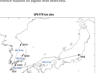
In the present study, a long baseline GPS RTK algorithm was directly developed; and to verify the performance of long baseline positioning using GPS dual frequency observation data, a total of four baselines were selected as shown in Fig. 2. All of the baselines were more than 100 km.
In particular, to verify the positioning performance of a very long baseline of more than 1,000 km, the Tsukuba (TSKB) GPS reference station in Japan was selected.
Table 1 summarizes the models used for the long baseline positioning. For the GPS observation data, code and carrier phase were used together; and the ionospheric error was eliminated by IF linear combination. Also, the tropospheric error was estimated epoch-by-epoch, and the earth tide loading effect (crust/ocean/pole) was considered because the GPS reference station and the user that were located on different crustal plates could have different motions when the baseline increased. The phase centers of the GPS satellite antenna and the receiver antenna and their variations were calculated, respectively, and were used for data processing. Lastly, the carrier phase wind-up effect due to the relative motion of the GPS satellites and the receiver was considered.
To verify the performance of the long baseline GPS RTK positioning, the observation data received at each GPS reference station on January 1, 2014 were used. The data processing was performed on a daily basis, and the state parameters were also calculated every 30 seconds. To reduce the effect of the orbital errors of the GPS satellites, the ultra-rapid product from the IGS was used.
Fig. 3 shows the position errors (i.e., each directional Fig. 2. The experimental sites for long baseline GPS RTK.
Fig. 3. The positioning errors of KOHG site estimated by GPS RTK.
Table 1. Data processing strategy of GPS RTK for long baselines.
Items Description
Processing filter Measurements Ionosphere Troposphere Tidal effect
Phase center offsets and Phase center variations Phase wind up
Extended Kalman filter
Code-carrier phase double difference Elimination by IF linear combination Estimation with GPT/GMF IERS conventions 2010 & FES2004 IGS08.atx
Wu et al. (1993)
GPT: global pressure and temperature, GMF: global mapping function, FES: finite element solutions, IERS: international earth rotation service
component) of the KOHG reference station calculated by the relative positioning between the Jeju (JEJU) and Goheung (KOHG) GPS reference stations. In this regard, the position information of the JEJU and KOHG reference stations (i.e., true values) were obtained using the Global Navigation Satellite System Precise Point Positioning (GNSS PPP) Software developed by the Korea Astronomy and Space Science Institute. In Fig. 3, the X-axis represents the Universal Time (UT), and the Y-axis represents the position error of the user. The calculated results were the mean and root mean square (RMS) values of the position errors during a day in the east-west, north-south, and up-down directions, respectively. The mean position errors of KOHG were less than 1 cm for every directional component, and the RMS values in the east-west, north- south, and up-down directions were 1.23 cm, 0.89 cm, and 2.55 cm, respectively. It is noteworthy that the positioning results were unstable at around 13:00 UT. This was because the number of common satellites between JEJU and KOHG
was less than four as shown in Fig. 4. During a day, the number of common satellites changed between 3 and 10, as shown in Fig. 4.
Fig. 5 shows the daily position errors of the BHAO GPS reference station calculated by the relative positioning between the JEJU and Bohyeonsan (BHAO) GPS reference stations. The baseline between JEJU and BHAO was about 393.37 km, and the mean position errors of BHAO in the east-west, north-south, and up-down directions were 0.15 cm, -1.33 cm, and -2.00 cm, respectively. Also, the RMS values for each component were 1.95 cm, 2.41 cm, and 3.65 cm, respectively. The RMS values of the BHAO were larger than those of the KOHG reference station, in every directional component. In particular, the RMS value in the up-down direction was the largest similar to the case of KOHG. In Fig. 6, the positioning results were instantaneously unstable at 13:00 UT. It is thought that the abrupt decrease in the number of common satellites at 13:00 UT shown in Fig. 6 affected the positioning results.
Fig. 4. Variations of the number of common GPS satellites between JEJU and KOHG. The red dot-circle represents less than four common satellites.
Fig. 3. The positioning errors of KOHG site estimated by GPS RTK.
Fig. 4. Variations of the number of common GPS satellites between JEJU and KOHG. The red dot- circle represents less than four common satellites.
Fig. 5 The positioning errors of BHAO site estimated by GPS RTK.
Fig. 5. The positioning errors of BHAO site estimated by GPS RTK.
Fig. 6. Variations of the number of common GPS satellites between JEJU and BHAO. The red dot- circle represents less than four common satellites.
Fig. 7. The positioning errors of SKCH site estimated by GPS RTK.
Fig. 6. Variations of the number of common GPS satellites between JEJU and BHAO. The red dot-circle represents less than four common satellites.
Fig. 6. Variations of the number of common GPS satellites between JEJU and BHAO. The red dot- circle represents less than four common satellites.
Fig. 7. The positioning errors of SKCH site estimated by GPS RTK.