Prediction of Serum Creatinine in Hemodialysis Patients Using a Kernel Approach for Longitudinal Data

(1)

I. Introduction

Chronic renal failure (CRF) is an irreversible kidney condi- tion that leads to end-stage renal disease (ESRD) [1]. ESRD patients require replacement interventions, such as kidney transplant or hemodialysis. Globally, ESRD is a substantial issue in the medical field. In the absence of replacement interventions for these patients, ESRD leads to death [2].

There were about 3,730,000 patients in ESRD by the end of 2016. Taiwan, Japan, and the United States have the highest ESRD prevalence in the world [3]. In Iran, ESRD prevalence is 610 per million people, which is greater than the global

Prediction of Serum Creatinine in Hemodialysis Patients Using a Kernel Approach for Longitudinal Data

Mohammad Moqaddasi Amiri¹, Leili Tapak^1,2, Javad Faradmal^2,3, Javad Hosseini¹, Ghodratollah Roshanaei^2,3

1Department of Biostatistics, School of Public Health, Hamadan University of Medical Sciences, Hamadan, Iran

2Modeling of Noncommunicable Diseases Research Center, Hamadan University of Medical Sciences, Hamadan, Iran

3Department of Biostatistics and Epidemiology, School of Public Health, Hamadan University of Medical Sciences, Hamadan, Iran

Objectives: Longitudinal data are prevalent in clinical research; due to their correlated nature, special analysis must be used for this type of data. Creatinine is an important marker in predicting end-stage renal disease, and it is recorded longitudinally. This study compared the prediction performance of linear regression (LR), linear mixed-effects model (LMM), least- squares support vector regression (LS-SVR), and mixed-effects least-squares support vector regression (MLS-SVR) methods to predict serum creatinine as a longitudinal outcome. Methods: We used a longitudinal dataset of hemodialysis patients in Hamadan city between 2013 and 2016. To evaluate the performance of the methods in serum creatinine prediction, the data was divided into two sets of training and testing samples. Then LR, LMM, LS-SVR, and MLS-SVR were fitted. The prediction performance was assessed and compared in terms of mean squared error (MSE), mean absolute error (MAE), mean absolute prediction error (MAPE), and determination coefficient (R²). Variable importance was calculated using the best model to select the most important predictors. Results: The MLS-SVR outperformed the other methods in terms of the least prediction error; MSE = 1.280, MAE = 0.833, and MAPE = 0.129 for the training set and MSE = 3.275, MAE = 1.319, and MAPE

= 0.159 for the testing set. Also, the MLS-SVR had the highest R², 0.805 and 0.654 for both the training and testing samples, respectively. Blood urea nitrogen was the most important factor in the prediction of creatinine. Conclusions: The MLS-SVR achieved the best serum creatinine prediction performance in comparison to LR, LMM, and LS-SVR.

Keywords: Creatinine, Support Vector Machine, Longitudinal Studies, Renal Dialysis, Machine Learning

Healthc Inform Res. 2020 April;26(2):112-118.

https://doi.org/10.4258/hir.2020.26.2.112 pISSN 2093-3681 • eISSN 2093-369X

Submitted: July 16, 2019 Revised: December 30, 2019 Accepted: March 19, 2020 Corresponding Author Javad Faradmal

Department of Biostatistics and Epidemiology, School of Public Health, Modeling of Noncommunicable Diseases Research Center, Hamadan University of Medical Sciences, Hamadan, Iran. Tel: +98- 9124055256, E-mail: javad.faradmal@umsha.ac.ir (https://orcid.

org/0000-0001-5514-3584)

This is an Open Access article distributed under the terms of the Creative Com- mons Attribution Non-Commercial License (http://creativecommons.org/licenses/by- nc/4.0/) which permits unrestricted non-commercial use, distribution, and reproduc- tion in any medium, provided the original work is properly cited.

(2)

average (580 per one million people) [3]. Seventy percent of ESRD patients receive hemodialysis treatment. Due to the 5%

to 6% annual increase in ESRD incidence and 1.1% increase in the global population, ESRD has become a major global health issues [3].

There is no indication in the early stages of CRF, and most of patients are identified in the end stage, in which the performance of the kidney has been totally disturbed. The accumulation of metabolic waste products occurs in CRF patients, which leads to changes in blood factors, such as serum creatinine. One way to diagnose patients with CRF is to check the serum creatinine [4,5].

In most clinical research, the outcome variable is collected longitudinally (multiple observations over time) for each patient or subject. For a longitudinal outcome, such as creatinine in CRF patients, the prediction of the actual values and checking their trend over time may be important. In longitudinal responses, due to unknown factors, the baseline value and the time trend of each patient may be different.

Therefore, to predict and analyze these responses, methods should be used that consider the differences in baselines and time trends. In other words, there is a correlation structure among the observations of the subject that needs to be considered in the modeling.

There are several methods for analyzing longitudinal responses, including the linear mixed-effects model (LMM), generalized liner mixed-effects model (GLMM), and generalized estimation equation (GEE) [6-8]. The most widely used method for continuous outcomes is LMM. This model is an extension of linear regression (LR) that considers the differences of baseline values and time trends using random effect terms. Linear or limited nonlinear relationships between covariates and response can be considered in LMM.

Therefore, LMM may not be useful in the presence of complex nonlinear relationships between outcome and features.

Recently, machine learning approaches have often been ap- plied to various prediction problems as classification or regression [9-11]. The least-squares support vector regression (LS-SVR) method is a machine learning approach that can be used for the prediction of continuous responses [12,13].

Complex nonlinear relationships between response and covariates can be considered in LS-SVR by using a kernel technique [12,14]. There have been a few studies that used the LS-SVR technique to predict longitudinal responses [14-17].

In this study, we used an LS-SVR method that takes into account random effects, in addition to complex relations.

We used a mixed-effects least-squares support-vector regression (MLS-SVR) method presented for longitudinal data sets

[15,16]. The aim of this study is to evaluate the prediction performance of LMM and MLS-SVR for serum creatinine.

To the best of our knowledge there has been no study that has used the LS-SVR method for CRF patients. Also we investigated the efficacy of random effects in the prediction of creatinine in hemodialysis patients. Obtaining the important variables in prediction of creatinine using the MLS-SVR method is another objective of this paper.

II. Methods

1. Data and Setting

We used a longitudinal dataset related to a study on hemodialysis patients in the hemodialysis department of Shahid Beheshti Medical Education Center of Hamadan city (Iran) between 2013 and 2016, which was collected for a master of science thesis [18]. There were 3,492 observations regarding 158 hemodialysis patients in the dataset. Some laboratory variables were collected longitudinally in the dataset, such as creatinine, fasting blood sugar (FBS), hematocrit (HCT), hemoglobin (HB), calcium (Ca), potassium (K), phosphorous (P), and blood urea nitrogen (BUN). Also, there were multiple fixed factors, such as the number of dialysis sessions in a week, gender, age, diabetes (yes or no), and hypertension (yes or no) in the dataset. We used the serum creatinine as the longitudinal response and the other variables as the fixed effects covariates. Also, the random intercept and trend were considered in the LMM and MLS-SVR methods as the random effects.

To evaluate the performance of the methods in the prediction of creatinine, the data was divided into two subsets, training and testing samples. Thus, because of the longitudinal nature of the data, the first 70% of observations related to each patient were considered as the training sample and the remainder were considered as the testing set. We fitted the LMM and MLS-SVR methods to the training and testing samples by considering the random intercept and trend in the models. Also, the LR model and ordinary LS-SVR were fitted to the data to assess the influence of taking into account random effects terms in the performance of the models in prediction of outcome. The data preprocessing is shown in Figure 1.

2. Classical Methods

LR and LMM are two classical models that were used in this study. The LR model is the most commonly used method for analyzing a continuous response variable with normal distribution. The effect of multiple covariates can be evaluated on

(3)

the response variable in LR models [19]. For a N × p covari- ate matrix (x0), the prediction function of LR is expressed as y(x0)= βˆ₀ + i x0i

∑

p

i=1

βˆ

(1)

where (β0,βi) are the regression parameters.

LR may not be useful when the dataset has a multilevel or longitudinal structure. There is a correlation structure in longitudinal data that needs to be taken into account in analysis. The LMM is an extended form of the LR model.

Random effects terms have been added to the LR for consideration of the correlation structure of the longitudinal data.

The LMM prediction function for a given data of (x0,z0) is obtained as

^ˆ^y(x0, z0) = ^β^ˆ0 + i x0i + vˆ '

∑

p

i=1

βˆ ⁱ

z

⁰ ₍₂₎

Here, (β0, βi) are the model’s fixed parameters related to the N × p covariate matrix (x0), and vi~N(0, ∑v) are the random effects parameters related to z0 which are the random effect variables.

3. Machine Learning Approaches

We used the ordinary LS-SVR and the MLS-SVR methods to predict serum creatinine. The LS-SVR model was explained by Suykens et al. [12] for regression problems in linear or nonlinear forms. The basic property of nonlinear LS-SVR is

the use of the kernel technique. The input data are mapped into a higher-dimensional space with kernel functions. Al- though a linear fitting is done in the new high-dimensional space, the fitting in the original input space is non-linear [20]. There are multiple kernel functions; the one that is most commonly used is the radial basis function (RBF) [12].

We used the RBF as the kernel function in this study. The prediction function of nonlinear LS-SVR for a given N × p matrix (x0) is introduced as

y(x0) = bˆ

αˆiK(x0, xi) + bˆ αˆ

∑

N

i=1 (3)

where (α,b) are the model parameters, and K(xi, xo) = φ'(xi) φ(x0) is the kernel function. Here, φ(.) is the nonlinear map- ping function, which is used in LS-SVR for nonlinear fitting of the data [12].

The MLS-SVR is the extended model of ordinary LS-SVR in which random effect terms are added for consideration of the correlation structure of the longitudinal data [16]. The MLS-SVR has the following prediction function for a given (x0, z0):

y(x0, z0) = bˆ αˆ

+ bˆ

αˆijK(xij, x0) + vˆ '

∑

N

i=1

∑

ⁿ

j 1=

z

0 (4)

i

Here, vi~N(0,∑v) are the random effects parameters related to the random-effects covariate matrix, and x0 is the fixed- effects covariate matrix, and K is the kernel function. Also, x_ij is the jth observation of the ith patient for j = 1, 2,…, ni

and i = 1, 2,…, N.

The parameters in the Equations (3) and (4) are estimated by constructing the Lagrange function and solving a linear system [12,14].

4. Evaluation Criteria

We evaluated the generalization performance of each model in the training and testing samples. Some criteria were used to compare the performance of the models, such as mean squared error (MSE), mean absolute error (MAE), mean absolute prediction error (MAPE), and determination coef- ficient (R²) as follows:

MSE =

∑

_{i 1}^N₌^(yⁱ–^yˆi)² (5)

N

MAE =

∑

_{i 1}^N₌^|yⁱ–^yˆi| (6)

N Data

collection

Data cleaning

Data transformation

Data analysis

Historical data collected from the

medical records for each patients

Excluding data with missing

values

Standardize each variable

Training and testing sets

LR, LMM, LS-SVR, and MLS-SVR

Figure 1. Framework of data pre-processing. LR: linear regres- sion, LMM: linear mixed-effects model, LS-SVR: least- squares support vector regression, MLS-SVR: mixed- effects least-squares support vector regression.

(4)

MAPE =

∑

^N_{i 1}₌^|yⁱ^–_y^yˆⁱ^| ₍₇₎

N i

R² = The square of correlation coefficient between y and yˆ (8) 5. Variable Importance

Evaluating the variable importance (VIMP) was another aim of this study. We used a permutation procedure with 100 iterations to specify the importance of each variable in predicting creatinine [21,22]. In the permutation procedure, one variable was permuted, and the others were fixed. The original MAE was obtained from the prediction of creatinine in the original dataset. Then each variable was permuted 100 times, and the new MAE was obtained from each permutation for each variable. The mean of differences between the new and the original MAEs was considered as the importance criterion.

III. Results

Among 158 hemodialysis patients in the study, 53.8% were male, 43% were hypertensive, and 39.9% were diabetic. Also, 58% of the patients were given dialysis three or four times in a week. The descriptive statistics of some variables of the patients are shown in Table 1.

The results of fitting the LMM for serum creatinine are displayed in Table 2. All of the independent variables were significant except the FBS and diabetes variables.

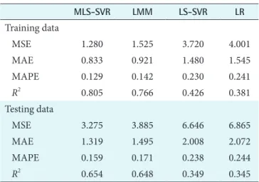
We used serum creatinine as the response variable. After dividing the longitudinal dataset into training and testing sets, we fitted the LR, LMM, LS-SVR, and MLS-SVR methods to the training set and investigated the fitting performance of each model. Then we evaluated the generalization performance of the models using the testing set. The results

are shown in Table 3.

As seen in Table 3, the MLS-SVR method achieved the best generalization performance based on all criteria. Also, there was a decrease in the prediction performance by ignoring the random effect terms in both LMM and MLS-SVR methods.

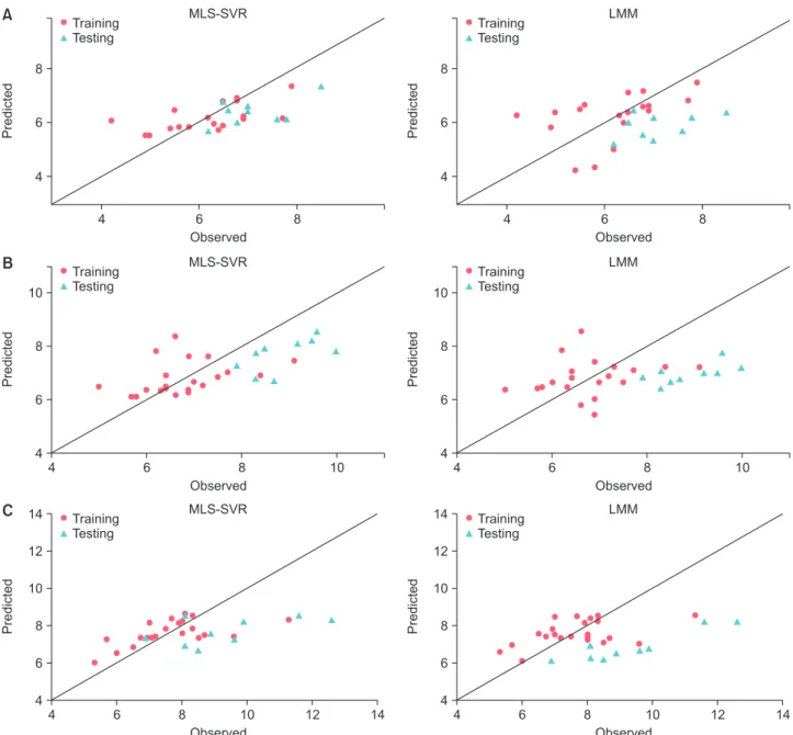
Figure 2 shows the observed versus predicted values of training and testing sets of 3 patients to compare the prediction performance of the MLS-SVR and LMM methods. As

Table 1. Descriptive statistics of hemodialysis data

Variable Male Female p-value

Creatinine 7.45 ± 3.13 6.99 ± 2.45 0.302 Blood urea nitrogen 130.06 ± 48.67 123.00 ± 43.08 0.335 Hematocrit 31.20 ± 5.79 32.00 ± 4.93 0.355 Hemoglobin 9.83 ± 2.05 10.01 ± 1.77 0.567 Fasting blood sugar 112.80 ± 50.11 108.71 ± 42.09 0.578 Potassium (K) 4.83 ± 1.00 4.93 ± 0.96 0.501 Phosphorous (P) 5.08 ± 1.65 5.09 ± 1.46 0.965 Calcium (Ca) 8.61 ± 1.28 8.95 ± 0.98 0.058

Age 59.19 ± 15.87 61.63 ± 14.93 0.321

Values are presented as mean ± standard deviation.

Table 2. Regression coeficient of covariates of fitting the linear mixed-effects model to serum creatinine

Variable Coefficient (standard error) p-value

Time 0.036 (0.010) 0.0002

Blood urea nitrogen 0.019 (0.001) <0.001

Hematocrit –0.038 (0.012) 0.001

Hemoglobin 0.208 (0.036) <0.001

Fasting blood sugar –0.001 (0.001) 0.312

Potassium (K) 0.129 (0.040) 0.001

Phosphorous (P) 0.172 (0.029) <0.001

Calcium (Ca) 0.086 (0.035) 0.015

Age –0.049 (0.023) <0.001

Diabetes (yes) 0.119 (0.256) 0.644

Gender (male) 0.616 (0.247) 0.014

Number of weekly dialysis 0.630 (0.216) 0.004 Hypertension (yes) 0.587 (0.254) 0.022

Table 3. Performance of the models in predicting creatinine for training and testing sets

MLS-SVR LMM LS-SVR LR

Training data

MSE 1.280 1.525 3.720 4.001

MAE 0.833 0.921 1.480 1.545

MAPE 0.129 0.142 0.230 0.241

R² 0.805 0.766 0.426 0.381

Testing data

MSE 3.275 3.885 6.646 6.865

MAE 1.319 1.495 2.008 2.072

MAPE 0.159 0.171 0.238 0.244

R² 0.654 0.648 0.349 0.345

MLS-SVR: mixed-effects least-squares support-vector regression, LMM: linear mixed-effects model, LS-SVR: least-squares support vector regression, LR: linear regression, MSE: mean squared error, MAE: mean absolute error, MAPE: mean abso- lute-prediction error, R²: determination coefficient.

(5)

seen, the prediction performance of the MLS-SVR method was better than that of LMM for both the training and testing data (the points in the MLS-SVR method were closer than those in the LMM method to the bisector line).

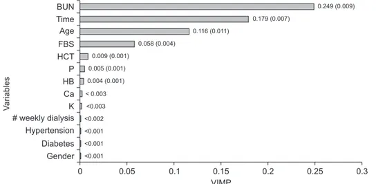
Finally, we obtained the VIMP (the mean of changes in MAE after permutation in each variable) in the prediction of creatinine using the MLS-SVR method (Figure 3). BUN, time, age, FBS, and HCT were the top rank variables among other variables. Indeed, there were more changes in the MAE criterion after the permutation of these variables.

IV. Discussion

In this study we compared the performance of four models in predicting the serum creatinine of hemodialysis patients by various random and fixed-effects approaches. The performance of both random effects models (MLS-SVR and LMM) was better than that of their fixed-effects counterpart models (LS-SVR and LM) in terms of generalization. It was demonstrated that random effect terms were effective in the prediction of creatinine and that they must be considered in the modeling process.

The MLS-SVR method achieved better performance than

4 8

6

4

6 8

Predicted

Observed MLS-SVR Training

Testing

4 8

6

4

6 8

Predicted

Observed Training LMM

Testing

4 8

6

4

6 8 10

Predicted

Testing

LMM

10

4 8

6

4

6 8 10

Predicted

Observed Training

Testing 10

4 8

6

4

6 8 10

Predicted

Testing

LMM

10

14 14

12

12 4

8

6

4

6 8 10

Predicted

Observed Training

Testing

10

14 14

12

A

B

C

Figure 2. Comparison of predicted and observed values for MLS-SVR and LMM for three patients: (A) patient #1, (B) patient #2, and (C) patient #3. The extended line is bisector. MLS-SVR: mixed-effects least-squares support-vector regression, LMM: linear mixed-effects model.

(6)

the LMM for both the training and testing datasets based on all criteria (Table 3). Figure 2 confirms this result, where the MLS-SVR achieved better performance for both training and testing samples for all 3 patients (the points are closer to the bisector line). Also, the prediction performance of the LS-SVR was better than that of the LR in the fixed-effects models (Table 2). Therefore, it is possible that there are complex or nonlinear relationships between some covariates and creatinine which the LMM and LR could not take it into account.

Limited studies have used support vector machine (SVM) approaches in the prediction of longitudinal continuous or categorical responses. In a study that compared several SVM methods for classification problems using simulation and real longitudinal data, the mixed-effects SVM achieved better performance than the other SVM models [23]. For a regression problem, Seok et al. proposed a mixed-effects LS- SVR. They used their proposed method for pharmacokinetic (PK) and pharmacodynamic (PD) datasets and compared their proposed model with the standard approach for the analysis of population PK and PD data. It was shown that the proposed MLS-SVR achieved the best performance for both training and testing data [16]. In another study that used the LS-SVR technique for longitudinal data, the LS-SVR method achieved better prediction performance than LMM in two real data examples and two simulation studies [14]. In a study on a three-level brucellosis frequency data, the MLS- SVR method achieved better prediction performance than the ordinary LS-SVR and classical models [15].

According to the variable importance that was calculated

using the random effects MLS-SVR, BUN was the most important variable in the prediction of the creatinine. Time, age, and FBS were the other variables that were important for creatinine prediction. Also, as seen in Table 2, BUN, HCT, HB, K, P, Ca, age, gender, number of weekly dialysis sessions, and hypertension had a significant effect on the value of serum creatinine. The age factor has been reported as a variable that affects serum creatinine [24,25].

In conclusion, our study showed that the MLS-SVR achieved the best performance in terms of generalization and that it could produce more accurate predictions of serum creatinine. Also, random effect terms had an impressive positive effect on prediction performance. Finally, in the presence of high dimensional or/and complex data-sets SVM approaches may be more useful than classical methods.

Conflict of Interest

No potential conflict of interest relevant to this article was reported.

Acknowledgments

This study was a part of PhD thesis of the first author in Biostatistics and funded by the Vice-Chancellor for Research and Technology of Hamadan University of Medical Sciences (No. 9609286041). Also, we thanks hemodialysis department of Shahid Beheshti Medical Education Center of Hamedan city.

Figure 3. Variable importance (VIMP) of each factor in prediction of creatinine using MLS-SVR method. Mean of changes in MAE af- ter each permutation (standard error). BUN: blood urea nitrogen, FBS: fasting blood sugar, HCT: hematocrit, P: phosphorous, HB: hemoglobin, Ca: calcium, K: potassium, MLS-SVR: mixed-effects least-squares support-vector regression, MAE: mean absolute error.

0 0.05 0.1 0.15 0.2 0.25

BUN Time Age FBS HCT P HB Ca K

# weekly dialysis Hypertension Diabetes Gender

0.3

Variables

VIMP

0.249 (0.009) 0.179 (0.007)

0.116 (0.011) 0.058 (0.004)

0.009 (0.001) 0.005 (0.001) 0.004 (0.001)

< 0.003

<0.003

<0.002

<0.001

(7)

ORCID

Mohammad Moqaddasi Amiri (http://orcid.org/0000-0002-8003-7123) Leili Tapak (http://orcid.org/0000-0002-4378-3143)

Javad Faradmal (http://orcid.org/0000-0001-5514-3584) Javad Hosseini (http://orcid.org/0000-0002-7029-1726) Ghodratollah Roshanaei (http://orcid.org/0000-0002-3547-9125)

References

1. Khazaei Z, Rajabfardi Z, Hatami H, Khodakarim S, Khazaei S, Zobdeh Z. Factors associated with end stage renal disease among hemodialysis patients in Tuyserkan City in 2013. Pajouhan Sci J 2014;13(1):33-41.

2. Bond M, Pitt M, Akoh J, Moxham T, Hoyle M, Ander- son R. The effectiveness and cost-effectiveness of methods of storing donated kidneys from deceased donors: a systematic review and economic model. Health Technol Assess 2009;13(38):iii-156.

3. The Iranian Dialysis Consortium. Iran Dialysis Calen- der [Internet]. Tehran, Iran: The Iranian Dialysis Con- sortium; c2019 [cited at 2020 Apr 28]. Available from:

http://www.icdgroup.org.

4. Zahran A, El-Husseini A, Shoker A. Can cystatin C re- place creatinine to estimate glomerular filtration rate? A literature review. Am J Nephrol 2007;27(2):197-205.

5. Lasisi TJ, Raji YR, Salako BL. Salivary creatinine and urea analysis in patients with chronic kidney disease: a case control study. BMC Nephrol 2016;17:10.

6. Hedeker D. Generalized linear mixed models. In: Everitt B, Howell DC, editors. 9780470860809. Hoboken (NJ):

John Wiley & Sons; 2005.

7. Hedeker D, Gibbons RD. Longitudinal data analysis.

Hoboken (NJ): John Wiley & Sons; 2006.

8. Verbeke G, Molenberghs G. Linear mixed models for longitudinal data. New York (NY): Springer; 2009.

9. Amini P, Ahmadinia H, Poorolajal J, Moqaddasi Amiri M. Evaluating the high risk groups for suicide: a comparison of logistic regression, support vector machine, decision tree and artificial neural network. Iran J Public Health 2016;45(9):1179-87.

10. Amini P, Maroufizadeh S, Hamidi O, Samani RO, Sepi- darkish M. Factors associated with macrosomia among singleton live-birth: A comparison between logistic regression, random forest and artificial neural network methods. Epidemiol Biostat Public Health 2016;13(4):

e11985.

11. Tapak L, Mahjub H, Hamidi O, Poorolajal J. Real-data

comparison of data mining methods in prediction of diabetes in iran. Healthc Inform Res 2013;19(3):177-85.

12. Suykens JA, Van Gestel T, De Brabanter J, De Moor B, Vandewalle J. Least squares support vector machines.

Singapore: World Scientific Publishing; 2002.

13. Suykens JA, Vandewalle J. Least squares support vector machine classifiers. Neural Process Lett 1999;9(3):293- 300.

14. Shim J, Sohn I, Hwang C. Kernel-based random effect time-varying coefficient model for longitudinal data. Neurocomputing 2017;267:500-7.

15. Amiri MM, Tapak L, Faradmal J. A mixed-effects least square support vector regression model for three-level count data. J Stat Comput Simul 2019;89(15):2801-12.

16. Seok KH, Shim J, Cho D, Noh GJ, Hwang C. Semipa- rametric mixed-effect least squares support vector machine for analyzing pharmacokinetic and pharmacodynamic data. Neurocomputing 2011;74(17):3412-9.

17. Amiri MM, Tapak L, Faradmal J. A support vector regression approach for three–level longitudinal data. Epi- demiol Biostat Public Health 2019;16(3):e13129.

18. Hosseini J. Comparison of longitudinal data analysis methods and its application in modeling health indica- tors [thesis]. Hamadan, Iran: Hamadan University of Medical Sciences; 2019.

19. Montgomery DC, Peck EA, Vining GG. Introduction to linear regression analysis. Hoboken (NJ): John Wiley &

Sons; 2012.

20. Vapnik V. The nature of statistical learning theory. New York (NY): Springer; 2010.

21. Zhang H, Singer BH. Recursive partitioning and appli- cations. New York (NY): Springer; 2010.

22. Sexton J. Historical tree ensembles for longitudinal data [Internet]. Wien, Austria: R Foundation; 2018 [cited at 2020 Apr 28]. Available from: https://cran.r-project.org/

web/packages/htree/htree.pdf.

23. Chen T, Zeng D, Wang Y. Multiple kernel learning with random effects for predicting longitudinal outcomes and data integration. Biometrics 2015;71(4):918-28.

24. Nguyen-Khoa T, Massy ZA, De Bandt JP, Kebede M, Salama L, Lambrey G, et al. Oxidative stress and haemo- dialysis: role of inflammation and duration of dialysis treatment. Nephrol Dial Transplant 2001;16(2):335-40.

25. Tatari M, Rahgozar M, Khanloo SA, Hosseinzadeh S.

The relationship between blood creatinine levels and survival of patients with kidney disease using joint longitudinal and survival model. J Health Promot Man- ag 2017;6(3):12-9.