A Study on CFD Analysis Methods using Francis-99 Workshop Model

◎ Original Paper

ISSN (Print): 2287-9706

A Study on CFD Analysis Methods using Francis-99 Workshop Model

Vu Le ^* ⋅Zhenmu Chen ^* ⋅Young-Do Choi ^**

^†

Key Words : CFD Analysis(CFD

), Francis-99 Workshop(

-99

), Losses Analysis(

), Performance(

), Pressure Distribution(

), Velocity Distribution(

)

ABSTRACT

The Francis-99 is a workshop initiated by the Norwegian University of Science and Technology (NTNU), Norway, and Lulea University of Technology (LTU), Sweden, in order to further validate the capabilities of the CFD technologies. The goal of the first workshop is to determine the state of the art of numerical predictions for steady operating conditions. When performing the CFD analysis, some geometry details are often neglected. In case of Francis Turbine, labyrinth seals are usually not include in the simulation domain, this may lead to inaccurate prediction of turbine efficiency. In this study, the CFD analysis for Francis-99 Workshop model has been performed for full domain of machine including top and bottom labyrinth seals. The efficiency value and distribution of velocity and pressure have been investigated and compared to the experimental data obtained from NTNU. By comparing the results, it was found that: With the top and bottom labyrinth seals in the domain, the CFD result was significantly improved in prediction of efficiency at all the operating point, especially at part load.

Fig. 1 Francis-99 workshop turbine test rig at the Waterpower laboratory, NTNU ⁽²⁾

1. Introduction

Computational fluid dynamics (CFD) is an established tool in industry for the design of Francis and other type of turbines. The principle task of the CFD tools is to predict the hydraulic efficiency and pressure distribution as accurately as possible and capture flow phenomena of importance.

⁽¹⁾

However, for reducing of computation time, some geometry details are often neglected. In case of Francis Turbine, labyrinth seals are usually not included in the simulation domain, this may lead to inaccurate prediction of turbine efficiency. In other studies of the Francis-99 workshop model, without labyrinth seals in domain, the difference between experimental and numerical efficiency at part load operating point is significant (14%).

⁽²⁾

In this study, the efficiency prediction is not only focused on, but also the velocity distribution and pressure distribution are investigated, and compared to experimental data obtained from NTNU.

2. Francis-99 workshop model and Numerical Model:

2.1 Francis-99 workshop model

The experimental data is obtained from the test rig

* Graduate School, Department of Mechanical Engineering, Mokpo National University, Mokpo.

** Department of Mechanical Engineering, Institute of New and Renewable Energy Technology Research, Mokpo National University, Mokpo.

† 교신저자(Corresponding Author), E-mail : [email protected]

Distributor (Spiral casing, guide vanes, stay vanes) 5,938,473

Runner 4,864,950

Draft tube 1,783,945

Top labyrinth seal 3,233,520

Bottom labyrinth seal 4,553,820

Total 20,374,708

Table 1 Mesh number of simulation domains

Fig. 2 Francis-99 workshop turbine numerical model

Fig. 3 Computation mesh of runner and labyrinth seals in detail

Parameter Part load BEP High load

Head [m] 12.29 11.91 11.84

Flow rate [m ³ /s] 0.071 0.203 0.221 Runner speed [rev/sec] 6.77 5.59 6.16 Guide vane angle [ ^o ] 3.91 9.84 12.44

Torque [N.m] 137.52 619.56 597.99

Efficiency [%] 71.69 92.61 90.66

Table 2 Operating conditions of the turbine by experiment

test rig model turbine is shown in Fig. 1. Experimental measurements were carried out using the open loop water circuit to get realistic conditions. Water from the basement was pumped to the overhead tank and flowed down to the upstream pressure tank connected to the turbine inlet pipeline. A uniform level of the water/head was maintained in the overhead tank at all operating points.

⁽²⁾

2.2 Numerical model and mesh

The computation domain consists of the spiral casing with stay vanes and guide vanes, runner, draft tube and also includes top and bottom labyrinth seals.

Simulation were performed on 2 types of mesh. First, the computation mesh was provided by organizers,

⁽³⁾

NTNU

MNU

NTNU

MNU

⁽⁴⁾

Structured hexahedral mesh is preferred over tetrahedral mesh because it gives faster convergence,

better quality and better results with less cells required. In

MNU

Fig. 2 shows the full simulation domain for Francis-99 workshop turbine model for CFD analysis.

A great care for labyrinth seal mesh is required. The mesh needs to cover all the detail of labyrinth seals and also the number of mesh should be as small as possible to reduce the computational cost. Table 1 shows the mesh number of simulation domains. In

MNU

Table 2 summarizes the operating conditions of the turbine and efficiency at each operating point by experiment. Mass flow rate and average pressure were prescribed at the inlet and outlet of simulation domain, using the normal method of other research results.

^(5-9)

NTNU

MNU

CC

⁽¹⁰⁾

Operating point

Mass flow rate [kg/s]

Volumetric loss [kg/s]

Proportion of Volumetric

loss [%]

Part load 70.95 0.44 0.61

BEP 202.84 0.43 0.21

High load 220.89 0.47 0.21

Table 4 Volumetric loss in labyrinth seals Cases Mesh Turbulece Model Labyrinth Seal

1 MNU SST Without

2 MNU SST With

3 MNU SST+CC With

4 NTNU SST With

Table 3 List of simulation conditions

Operating

point Cases Torque on the Shaft by CFD [N.m]

Torque_CFD/

Torque_Exp

Part load

1 171.55 1.25

2 140.18 1.08

3 139.60 1.08

4 162.53 1.18

BEP

1 666.96 1.08

2 645.58 1.04

3 645.40 1.04

4 657.55 1.06

High load

1 621.11 1.04

2 594.99 1.00

3 588.69 1.00

4 609.10 1.02

Table 6 Comparison of torque on the shaft with labyrinth seals Operating point Torque loss in top

labyrinth seal [N.m]

Torque loss in bottom labyrinth seal [N.m]

Part load 7.35 7.99

BEP 5.22 5.56

High load 6.22 6.78

Table 5 Torque loss in labyrinth seals

Fig. 5 Comparison of numerical torque to the experimental torque Fig. 4 Velocity distribution in runner and labyrinth seals

useful in tackling problems in high swirling flows. One case with the

CC

SST

Table 3 shows 4 cases of simulation condition, which were performed at each operating points to investigate the influence of labyrinth seals for efficiency prediction and comparison of mesh and turbulence model.

3. Results and Discussion

3.1 Volumetric losses and torque losses

The losses in labyrinth mainly consists of volumetric loss and torque loss. The volumetric loss at all operating points is very small due to no balance hole in runner.

Table 4 shows the result of volumetric loss in

labyrinth seals. The largest of proportion of volumetric loss is 0.61% at Part load, while at BEP and High load the proportions are 0.21%. Velocity distribution in runner and labyrinth seals is shown in Fig. 4.

Table 5 shows the results of torque loss in labyrinth seals at several operating points. At part load, the largest loss in top labyrinth and bottom labyrinth seals was found.

The difference between

NTNU

MNU

MNU

Operating

point Cases Numerical Efficiency [%]

Difference between numerical and

experimental Efficiency [%]

Part load

1 80.1 8.4

2 73.3 1.6

3 72.6 0.9

4 75.1 3.4

BEP

1 94.2 1.6

2 92.9 0.3

3 92.8 0.2

4 93.0 0.4

High load

1 93.1 2.5

2 91.2 0.5

3 91.3 0.6

4 92.4 1.7

Table 7 Results of efficiency prediction

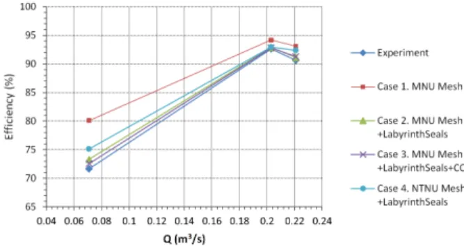
Fig. 6 Hill chart of the experiment Fig. 7 Comparison of numerical and experimental efficiency

the shaft predicted by

NTNU

MNU

NTNU

CC

CC

3.2 Efficiency prediction

The efficiency of Francis hydro turbine is calculated

by the equation:

   





Where,

η

T

ω

ρ

g

Q

H

Fig. 6 shows the hill chart of the experiment. Table 7 and Fig.7 shows the results of efficiency prediction with several simulation conditions at each operating point. From the results it is clear that the efficiency prediction is strongly influenced of labyrinth seals.

With the top and bottom labyrinth seals in simulation domain, the efficiency difference becomes lower down from 8.4% to 1.6% at part load, at BEP and high load the differences are 0.3% and 0.5%, respectively. The results at part load and high load were more improved with CC advance turbulence option (Case 3), while at high load the difference slightly increased. By comparing the results between Cases 2 and 4, the refinement at runner blades significantly improved the efficiency prediction by correcting the torque of runner shaft.

3.3 Velocity distribution validation:

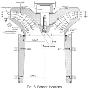
The Francis-99 workshop provided velocity data by experiment to validate the velocity distribution of numerical results. Velocity measurements (axial and tangential) were performed with a laser Doppler anemometer (LDA) along two horizontal lines in the draft tube. The two lines are located 64mm and 382mm below the draft tube inlet, respectively. The locations of velocity sensors were shown in Fig. 8 and Table 8.

Fig. 8 Sensor locations

Line 1 Line 2

Point 1 Point 2 Point 1 Point 2

x[m] -0.1789 0 0 -0.1965

y[m] 0 0 0 0

z[m] -0.2434 -0.2434 -0.5614 -0.5614

Table 8 Velocity sensor locations

Fig. 9 Part load: Velocity distribution at Line 1

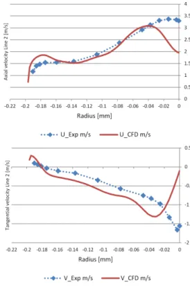
Fig. 10 Part load: Velocity distribution at Line 2

Fig. 11 BEP: Velocity distribution at Line 1

The validation of velocity distribution were performed for Case 2 (MNU mesh with top and bottom labyrinth seals).

Figs. 9 and 10 show the velocity distribution along

Line 1 and Line 2 at part load. The results of CFD analysis predicted similar results for the axial and tangential velocity along the radius. At Line 2, the axial velocity slightly overestimated and the tangential

Fig. 12 BEP: Velocity distribution at Line 2

Fig. 13 High load: Velocity distribution at Line 1

Fig. 14 High load: Velocity distribution at Line 2

velocity slightly underestimated compared to the measurement data.

The velocity results at design point are shows in Figs. 11 and 12. The CFD analysis results is fairly close to the experimental results of the axial velocity. However,

the results of CFD analysis clearly overestimate the tangential velocity close to the center.

At high load, the results of CFD analysis underestimate the axial velocity at both two Lines and overestimates the tangential velocity at Line 2 at the area close to the center, as shown in Figs. 13 and 14.

The CFD analysis overestimates the velocity close to the center of the runner. It can be conjectured that the runner cone and bolt give effect on the flow velocity as shown in Fig. 8, because the runner cone and the bolt was not considered in the CFD analysis domain.

Therefore, the CFD results over estimate the velocity at this part.

3.4 Pressure distribution validation

Pressure measurement were obtained at 6 locations at each operating point. The exact position of the pressure sensors are presented in Fig. 8 and Table 9.

The numerical results obtained with Case 2 (MNU mesh with top and bottom labyrinth seals) were compared with measurement data.

Fig. 15 presents pressure distribution at part load operating point. The results at VL01, DT11 and DT21 are very close to the experiment data, while the

VL01 P42 S51 P71 DT11 DT21 x[m] 0.2623 7.16E-5 -0.0800 -0.1965 -0.0904 0.0904 y[m] 0.1935 0.1794 0.0838 0 0.1566 -0.1566 z[m] -0.0296 -0.0529 -0.0509 -0.5614 -0.3058 -0.3058

Table 9 Pressure sensor locations

Fig. 15 Pressure distribution at part load

Fig. 16 Pressure distribution at BEP

Fig. 17 Pressure distribution at high load

maximum difference observed in pressure side of a blade (P42, 9.56%). In case of BEP, the better agreement between numerical and experimental values was obtained as shown in Fig. 16. At all pressure sensors the differences are lower than 2.96%.

At high load, the average pressure difference in the location of VL01 is 3.46% and the numerical pressure is lower than the measured pressure. In draft tube, the differences between the numerical and measured values at DT11 and DT21 are 7.02% and 6.21%, respectively. The best agreement of pressure between experiment and simulation is obtained in suction side of a runner blade (S51).

4. Conclusion

In present study, the CFD analysis for Francis-99 workshop turbine has been performed for full domain

including top and bottom labyrinth seals. The efficiency values and distribution of velocity and pressure have been investigated and compared to the experimental data obtained from

NTNU

The efficiency prediction at part load was more improved by including CC advance turbulence option.

The difference between numerical and experimental efficiency at part load become lower down from 1.61%

to 0.89%. The influence of refinement mesh at runner blades is significant. The coarse mesh in runner of NTNU mesh leads to overestimation of the torque in runner shaft and the efficiency, which are higher than those of experiment.

The distributions of velocity and pressure also were investigated in this study. The CFD analysis can predict accurate results for the axial and tangential velocities along the radius. However, the results of CFD analysis often overestimate or underestimate the axial and tangential velocities at the region close to the center. From the results of pressure distribution, numerically predicted pressures at six locations were compared to the measured results and showed the correct prediction, especially at BEP.

Acknowledgments

This work was supported by the New and Renewable Energy of the Korea Institute of Energy Technology Evaluation and Planning (KETEP) grant funded by the

Korea government Ministry of Trade, Industry and Energy (No. 2013T100200079).

References

(1) Wallimann, H., and Neubauer, R., 2015. “Numerical Study of a High Head Francis Turbine with Measurements from the Francis-99 Project,” In Journal of Physics, Vol. 579, No. 1, p. 012003.

(2) Trivedi, C., Cervantes, M. J., Gandhi, B. K., and Dahlhaug, O. G., 2013, “Experimental and Numerical Studies for a High Head Francis Turbine at Several Operating Points,” The American Society of Mechanical Engineers Journal of Fluid Engineering, Vol. 135, No.

11, 111102.

(3) NTNU and LTU Francis-99 test case http://www.

ltu.se/research/subjects/Stromningslara/Konferenser/Fra ncis-99/Test-Case-1.111520?l=en.

(4) ANSYS Inc, 2013, “ANSYS CFX Documentation” Ver.

15, http://www.ansys.com.

(5) Wu, J., Shimmei, K., Tani, K., Niikura, K., and Sato J., 2007, “CFD Based Design Optimization for Hydro

Turbines,” The American Society of Mechanical Engineers Journal of Fluids Engineering, Vol. 129, No.

2, pp. 159∼168.

(6) Wu Y., Liu S., Wu X., Dou H., Zhang L., and Tao X., 2010, “Turbulent Flow Computation Through a Model Francis Turbine and Its Performance Prediction,” Earth and Environmental Science, Vol. 12, No. 1, p. 012004.

(7) Cervantes M. J., Andersson U., and Lovgren H. M., 2010, “Turbine-99 Unsteady Simulations-Validations,”

Earth and Environmental Science, Vol. 12, p. 012014.

(8) Zhang, L. X., Wang, W. Q., and Guo, Y., 2007,

“Intrinsic Features of Turbulent Flow in Strongly 3-D Skew Blade Passage of a Francis Turbine,” Journal of Hydrodynamics, Vol. 19, No. 1, pp. 92∼99.

(9) Buntić O. I., Dietze S., and Ruprecht A., 2005,

“Numerical Simulation of the Flow in Turbine-99 Draft Tube,” In Proceedings of the Third IAHR/ERCOFTAC Workshop on Draft Tube Flow, Porjus, Sweden, pp. 8∼9.

(10) Smirnov, P. E. and Menter, F., 2009, “Sensitization of

the SST Turbulence Model to Rotation and Curvature

by Applying the Spalart-Shur Correction Term,” Journal

of Turbomachinery, Vol. 131 No. 4, p. 041010.