Multi-Objective Design Optimization of Composite Stiffened Panel Using Response Surface Methodology

Paper

Multi-Objective Design Optimization of Composite Stiffened Panel Using Response Surface Methodology

Mohanraj Murugesan *, Beom-Soo Kang*, Kyunghoon Lee**

ABSTRACT: This study aims to develop efficient composite laminates for buckling load enhancement, interlaminar shear stress minimization, and weight reduction. This goal is achieved through cover-skin lay-ups around skins and stiffeners, which amplify bending stiffness and defer delamination by means of effective stress distribution. The design problem is formulated as multi-objective optimization that maximizes buckling load capability while minimizing both maximum out-of-plane shear stress and panel weight. For efficient optimization, response surface methodology is employed for buckling load, two out-of-plane shear stresses, and panel weight with respect to one ply thickness, six fiber orientations of a skin, and four stiffener heights. Numerical results show that skin-covered composite stiffened panels can be devised for maximum buckling load and minimum interlaminar shear stresses under compressive load.

In addition, the effects of different material properties are investigated and compared. The obtained results reveal that the composite stiffened panel with Kevlar material is the most effective design.

Key Words: Multi-objective optimization, Response surface methodology, Buckling load, Out-of-plane shear stress

1. INTRODUCTION

Stiffened composite panel (SCP) applications in the field of aerospace have significantly increased in the last decade [1]. In SCP design, the buckling phenomenon, which ends up in a large-scale transverse deflection under compressive load, is the primary criterion [1]. For efficient laminate design, factors such as a fiber orientation, a thickness, and the number of lay- ers need to be meticulously examined. Researchers have adopted several approaches to solve the above mentioned con- siderations. A laminate design problem can be characterized as a non-linear, multi-model, and multi-dimensional problem, and design parameters include both discrete and continuous variables [2,3]. This research is committed to the optimal design of an SCP that is predominantly used in aircraft parts, such as a fuselage and wing panels.

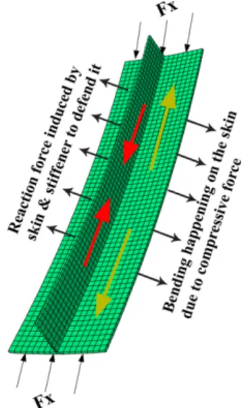
The buckling stability of an SCP requires one to take into account of compression, shear, and combined compression- shear loads. Under these load cases, stiffened composite panels usually experience local skin buckling, stiffener buckling, and global buckling. The failure of an SCP often starts at the inter-

face between a skin and stiffeners because of stress concen- tration induced by different skin and stiffener deformation after local skin buckling [4,5]. This failure mode generally hap- pens as a result of delamination, and it arises due to the pres- ence of inter-laminar shear stress in the laminates and limitation on adhesive bonding strength [6,7].

To enhance the buckling load of an SCP, we draw on the use of a cover skin. A cover skin enlarges the contact area between a skin and stiffeners, which leads to bending stiffness increase given compressive load. This design strategy is based on knowledge about how the failure of an SCP initiates at the interface between a skin and stiffeners after local skin buck- ling. In this study, we deal with only pre-buckling phenom- enon owing to the snag of a buckling phenomenon in composite structures. For an SCP, we consider those made up of straight shaped, T-shaped, and L-shaped stiffeners.

Stiffened panel design problem typically requires expensive computational efforts. To overcome this difficulty, we exploit design optimization based on surrogate modeling. A surrogate model can replace an expensive simulation model during the preliminary design and optimization process [8]. In the lit-

Received 6 July 2015, received in revised form 27 October 2015, accepted 28 October 2015

*

**

Department of Aerospace Engineering, Pusan National University

Department of Aerospace Engineering, Pusan National University, Corresponding author (E-mail: [email protected])

erature, Luca et al. [9,10] inspected their problem with arti- ficial neural networks aiming at the weight minimization of an SCP. Rikards et al. [11,12] examined their problem with response surface methodology (RSM) to derive the prelimi- nary design guidelines of an SCP under post-buckling con- straints. On the other hand, both experimental and numerical results were used for the construction of a surrogate model.

Akula [13] investigated the influence of fiber and matrix prop- erties on the structural response of a composite panel. There- after, a radial basis function model is constructed for reliability analysis. We tackle our problem with RSM to design an SCP that is able to work under compressive load.

In this research, a response surface model is built with sim- ulation data based on a computer experiment, and the fitness of the constructed models is verified. Polynomial models obtained by RSM are used as objective functions for our design problem. A multi-objective optimization problem is formulated for the maximum buckling load by minimizing both maximum out-of-plane shear stress and panel weight in MATLAB. The SCP design variables are one ply thickness, six fiber orientations of skin, and four stiffener heights. For the identification of the best design among optimal designs, the technique for order preferences by similarity to ideal solution (TOPSIS) is adopted. Overall, this paper seeks for the best SCP design with different materials in consideration of buckling load, interlaminar shear stress, and panel weight.

2. STIFFENED PANEL DESIGN FORMULA- TION

2.1 Model Description

A finite element model of an SCP is built in ANSYS as shown in Fig. 1. In order to address an SCP design problem, we utilized a computer experiment for surrogate model con- struction. We consider a stiffened panel of size 356 × 356 mm

, which is bent to form a cylindrical surface with a radius of

381 mm [14]. We chose this panel configuration because this shape had been employed by previous researchers [11,12].

This panel is supported by four stiffeners located symmetri- cally with a distance of 89 mm between two stiffeners. The panel skin edges A and C are loaded by uniform compressive load F

= 20,000 N, and it is restrained in displacement U

= U

= 0 and in rotation about R

= R

= R

= 0. Two lon- gitudinal edges B and D are restrained in displacement and in rotation like edges A and C. For an initial configuration, the skin has a stacking sequence of [0/45/90]

. For the entire case, the stiffener has a fixed stacking sequence of [45/-45/90/0/0/

90/-45/45]

. In this research, three stiffener shapes are counted for numerical investigation as illustrated in Fig. 2: a flat sec- tion, a T section, and an L section. A cover skin is made up of the same material as a skin, and two layers are placed in [-45/

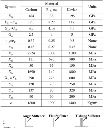
45] orientations. The material ply thickness is 0.125 mm, and epoxy is used for resin/matrix. The properties of the three materials are listed in Table 1.

2.2 Numerical Model

The critical buckling behavior of an SCP is modeled in ANSYS as a linear eigenvalue problem. Composites are typ- ically thin walled structures, thus we modeled the panel with a linear shell element. In this paper, the cover skin approach assumed that the cover skin is perfectly bonded to the skin and Fig. 1. Finite element model of an SCP

Table 1. Material properties of composite panel

Symbol Material

Units Carbon E-glass Kevlar

E

164 38 195 GPa

E

=E

12.8 8.27 14.6 GPa

G

=G

4.5 4.14 7.5 GPa

G

2.5 4 5 GPa

υ

=υ

0.32 0.25 0.3 None

υ

0.45 0.27 0.45 None

X

2724 1050 3100 MPa

X

111 690 500 MPa

X

50 55 150 MPa

X

1690 140 1800 MPa

X

=X

290 275 600 MPa

S

120 70 250 MPa

S

137 80 320 MPa

S

90 60 200 MPa

ρ 1800 1900 1400 Kg/m

Fig. 2. Stiffened panel with multiple stiffener shapes

stiffeners as shown in Fig. 3, Fig. 4, and Fig. 5. A multi-point constraint is employed for both skin/stiffener and web/flange assemblies such that they are perfectly bonded with no sep- aration.

2.2.1 Linear Elasticity Analysis

In this present study, four-noded element with six degrees of freedom at each node termed as SHELL181 is chosen. The computation for the four-noded shell element is governed by first order shear deformation theory (FSDT). The theory has the capability of evaluating from thin shell to substantially thick shell structures. The theory can also deal with the non- linear analysis of thin plates [15] and interlaminar shear stress at the layer interfaces. To obtain the interlaminar shear stress, we can use output definitions (ILSXZ, ILSYZ); here, ILSXZ and ILSYZ denote the interlaminar shear stress components in xz and yz plane.

The kinematic assumptions of FSDT are as follows:

(1)

where u, v and w represents the displacements. The in-plane displacements are u

, v

, whereas the transverse displacement of the mid-plane is w

. The rotations of normal to mid plane about y and x axes are θ

and θ

, respectively, and θ

is the higher order terms in Taylor’s series expansion.

The displacement δ can be expressed in terms of shape functions N

as

(2)

where , φ represents the rota-

tion compoenents in each node for all the three axis.

Four noded shell elements represented in natural coordi- nates (ξ−η) is given as

(3)

where N

to N

are the shape functions. Strains are obtained by derivation of displacements as

(4)

where . Here a comma fol-

lowed by a subscript denotes partial differentiation. The nor- mal strain components of in plane direction are u

, v

and w

. The shear strain components of out of plane direction are u

, v

, v

, w

, w

, and u

. The strain vector can be expressed in terms of a nodal displacement vector such that

(5) where [B] is the strain displacement matrix containing inter- polation functions and their derivatives, and {δ} is the nodal displacement vector. The generalized stress-strain relationship with respect to its reference plane can be expressed as

(6)

where {σ} and {ε} are the stress and strain vector, respectively, and [D] is the rigidity matrix. Using the virtual work method, element stiffness matrix [K

] can be derived as

u x y z ( , , ) u =

( x y , ) zθ +

( x y , ) v x y z ( , , ) v =

( x y , ) zθ +

( x y , ) w x y z ( , , ) w =

( x y , ) zθ +

( x y , )

⎩ ⎪

⎨ ⎪

⎧

δ N

δ

∑

=

δ

= [ u

v

w

φ

φ

φ

]

N

1

4 -- 1 ξ ( – ) 1 η ( – )

= N

1

4 -- 1 ξ ( + ) 1 η ( – )

= N

1

4 -- 1 ξ ( + ) 1 η ( + )

= N

1

4 -- 1 ξ ( – ) 1 η ( + )

⎩ =

⎪ ⎪

⎪ ⎪

⎨ ⎪

⎪ ⎪

⎪ ⎧

ε

{ } = { u

v

w

u

+v

v

+w

w

+u

}

ε

{ } = { ε

ε

ε

r

r

r

}

ε

{ } = [ ] δ B { }

σ

{ } = [ ] ε D { } Fig. 4. L-shape stiffened panel with cover skin

Fig. 5. T-shape stiffened panel with cover skin

Fig. 6. Forces acting on the stiffened panel

Fig. 3. Flat shape stiffened panel with cover skin

(7)

where |J| is the determinant of the Jacobian matrix.

The deflections can be resolve for static analysis as follows:

(8) where {P} is the static load column vector.

2.2.2 Linear Buckling Analysis

Linear buckling analysis predicts the buckling strength of linear elastic structure. It is assumed that structure configu- ration has no change in the process of loading. The buckling load is taken as the load when the determinant of stiffness matrix becomes zeros. Eigenvectors corresponding to an unstable state are calculated [16].

The buckling problem is formulated as an eigenvalue problem:

(9) where K

, K

and λ

represents the initial stiffness matrix, the stress stiffness matrix, and the buckling load factor, respectively.

The Critical buckling load P

can be obtained through the equation:

(10) where P is the design service load.

2.2.3 Stiffened Panel Weight Calculation

The weight of the SCP is calculated directly from ANSYS that produces the weight to area ratio n for ply material based on given ply thickness as given below:

(11) where . Symbol ρ denotes the density of ply material and t denotes the thickness of ply. Subsequently, the covered ply area is calculated after the composite modeling process.

Then, the weight to area raito is used for the calculation of the panel weight as shown below:

(12) where A is the covered ply area of the stiffened panel.

2.3 Design Optimization Formulation

The present investigation is concerned with the multi objec- tive optimization of a composite stiffened panel. An optimi- zation problem is formulated for maximum critical buckling load (P

) by minimizing both maximum out-of-plane shear stresses (τ

, τ

), and the panel weight (w) over choosing appropriate design variables.

The multi-objective optimization problem can be expressed as follows:

Minimize:

subjected to ,

where x is the vector of design variables, n is number of vari- ables, and LB and UB stand for lower bound and upper bound of input parameters.

3. SURROGATE MODELING

3.1 Response Surface Method

Response surface methodology (RSM) is a statistical tech- nique used in the development of a functional relationship between a response of interest, y, and a number of associated control (or input) variables denoted by x

, x

,…, x

. A response surface model can be written in the form such that [17]:

(13) where ε is called the error term, disturbance term, or noise.

This variable captures other factors that affect the response y other than the control variables x

.

In RSM, the form of a relationship between the response and the independent variable is unknown. Thus the first step in RSM is to find a suitable approximation for the true func- tional relationship between approximating function and true response function. Usually a second order model is utilized in RSM to approximate the function as follows [17,18]:

(14)

In equation (14), β

is called the intercept, whereas β

, β

, and β

are the regression coefficients of quadratic model, and k is the total number of samples.

The observation response vector y at n data point of func- tion y can be written in matrix notation as follows [18]:

(15) In equation (15), X is a matrix of the control variables and β is a vector of the regression coefficients.

The least squares method, which is minimizing the sum of the squares of random errors, is used for the estimation of unknown vector β. Therefore, the estimated vector β can be written as [18]:

(16)

3.2 Sampling Plan

The design of experiments is an efficient procedure that aims to gather as much information as possible with as little effort as possible. The design of experiments is conducive for the determination of an input/output relationship with sur- rogate modeling methods. An important issue in surrogate modeling is how to achieve reliable surrogates with a rea- K

[ ] [ ] B

[ ] B D [ ] J dedn

–1 +1 1

∫

– +1

∫

=

K

[ ] δ { } = { } P

K

[ ] λ +

[ ] K

( ) δ { } 0 =

P

= λ

× P

n = w/A n = ρ t ×

w = n A ×

f

( ) x

– , f

( ) f x ,

( ) f x ,

( ) x

( )

x

< < x

x

i = 1 …n

y = f x (

, , , x

… x

) ε +

y β

β

x

i 1=

∑

^β

^x

∑

^β

^x

^x

^{+ ε}

∑

∑

+ + +

=

y = X β ε +

βˆ = ( X

X )

X

y

sonable number of samples. For an experimental design with RSM, a central composite design (CCD) with face centering was employed. According to the chosen sampling scheme, a total of 151 computer experiments is required for the 11 fac- tors in Table 2; one sample at the center of an 11-dimensional hypercube, 22 samples at –α/+α coordinates along each axis of the hypercube, and 128 samples by a 2

fractional factorial design. In addition to the 151 sample generation, extra 151 samples are randomly generated for the verification of fitted response surface models.

3.3 Numerical and Graphical Verification

We are required to verify whether the predictions of the fit- ted surrogates are good or not. There are various metrics for the evaluation of surrogate model accuracy. In this study, the model adequacies were checked by the coefficient of deter- mination R

, an adjusted-R

, and a root mean square error (RMSE).

3.3.1 R-squared

It measures how much variability in an observed response can be accounted for by a fitted surrogate model. It typically ranges from 0 to 1. A good surrogate model will have a large R

that lies in-between 0.95 to 1.

(17)

3.3.2 Adjusted-R

It is a modified version of R-squared that has been adjusted for the number of control/input variables in the model. It is necessary for checking the adjusted R

because it adjusts the statistic based on the number of independent

variables in the model.

Adjusted - R

= (18)

3.3.3 Root Mean Square Error (RMSE)

It is the square root of a mean squared error. It is a measure of the differences between observed data and predicted data by a surrogate. The smaller value implies how closer the fit is with respect to the observation.

(19)

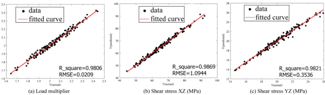
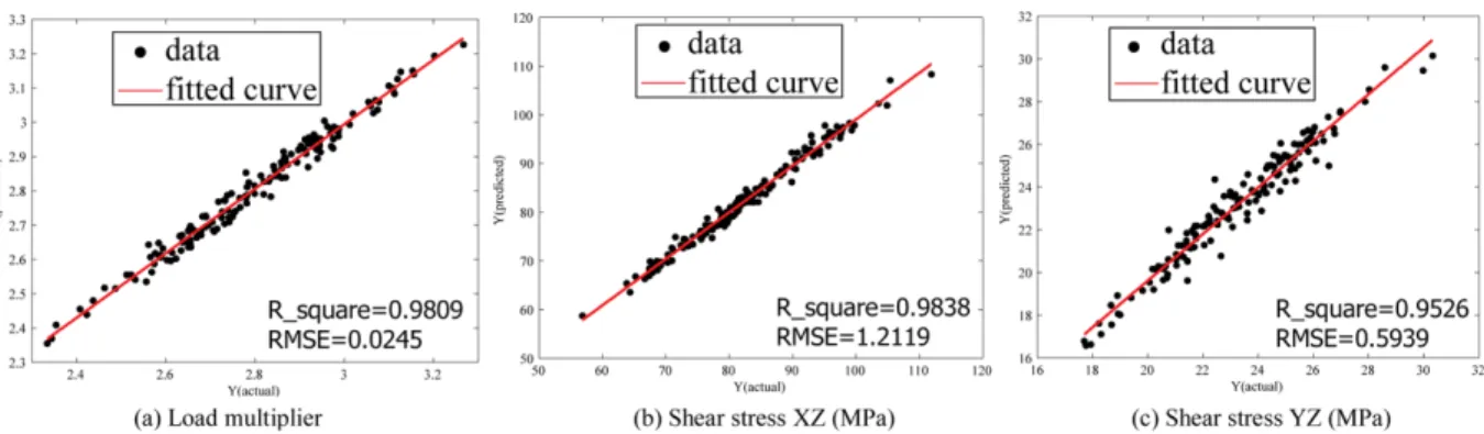
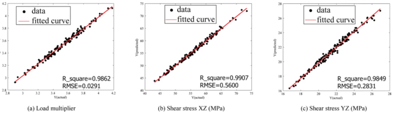
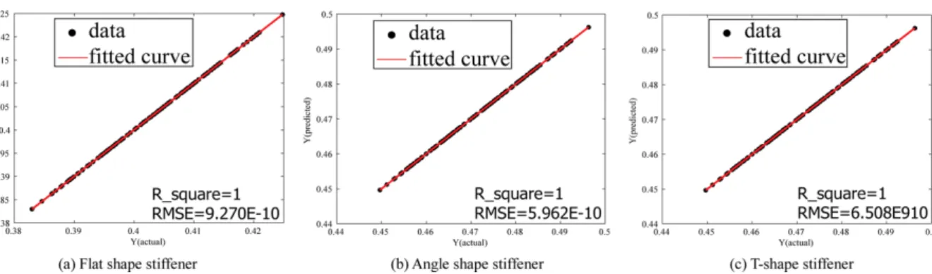
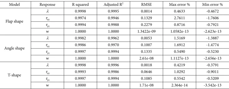
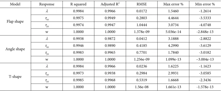
3.4 Verification Results

Numerical metrics for verification are evaluated with the CCD samples and summarized in Table 4, Table 5, and Table 6. High values of R

indicate that the fitted regression models well align with the observed data. In Table 4 to Table 6, we can see that adjusted-R

values are almost the same as R

values, but they are slightly less, which typically occurs as the number of input variables increases. In the tables, RMSE shows the overall closeness of the fitted regression models to the observed data. In sum, the fitted quadratic models are quite accurate compared to the observed data. Apart from the numerical verification, graphical verification is performed with the random samples as shown in Fig. 7 to Fig. 18. The fig- ures illustrate predicted data by surrogates against the actual data by ANSYS simulation. For the random samples, R- squared values range from 0.95 to 1.0, which conveys that the fitted surrogates are quite good at predicting responses at unseen inputs. After confirmation runs with the random sam- ples, we are good to use the fitted regression models as objec- tive functions to address a multi-objective problem for SCP design.

3.5 Optimization Procedure

The regression models obtained with RSM are used as objective functions. The genetic algorithm (GA) is employed in this work for multi-objective optimization. The GA is one of the most prominent methods that have been extensively used for SCP design optimization. Although the GA is a popula- tion-based approach and generally is able to prevent the search procedure from being trapped in local optima. We used a population size of 200 with the maximum generation of 2,200.

A Pareto fraction and a distance function is used for the control of the elitists of the genetic algorithm. We set the Pareto fraction to 0.5, which is 50% of the population size.

After multi-objective optimization with the GA, the best alternative, nearest to the positive ideal solution among Pareto optimal samples, has been identified with TOPSIS.

R

1

y

– yˆ

( )

∑

y

– y ( )

∑

--- –

=

1

y

– yˆ

( )

∑

y

– y ( )

∑

--- –

RMSE

yˆ

– y

( )

i 1=

∑

--- n

= Table 2. Design spaces of design variables in optimization

Process variables Input parameter

Lower bound

Upper bound

Stiffener height 1 X

22 25

Stiffener height 2 X

22 25

Stiffener height 3 X

22 25

Stiffener height 4 X

22 25

Ply thickness X

0.125 0.135

Ply angle 1 X

-45 0

Ply angle 2 X

0 45

Ply angle 3 X

60 90

Ply angle 4 X

60 90

Ply angle 5 X

0 45

Ply angle 6 X

-45 0

4. RESULTS AND DISCUSSION

Numerical investigation of an SCP was conducted for the three stiffener shapes and for the three different material prop- erties. After optimization with surrogates, extra numerical investigation was performed with ANSYS simulation for the validation of the optimization results with surrogates. The optimization results in Table 7 to Table 10 show that the values predicted by regression models and those predicted by the original ANSYS simulation are slightly different. In Table 7 to Table 10, the maximum errors do not exceed 2.586%, which assures that optimization with surrogates are credible.

In Table 7, optimization results are presented for the critical buckling load objective with carbon fiber material. The results show that the critical buckling load for the panel with flat shape stiffeners is 48.208 KN; on the other hand, those with the angle shape and T-shape stiffeners are 65.176 KN and 72.808 KN, respectively. Among the three stiffeners, the T-shape stiffener is found to carry the ultimate buckling load when all the panels are made of the same material. The panel with T- shape stiffener provides the maximum critical buckling load because this panel possesses high bending stiffness that offers resistance to bending deformation. As the bending stiffness depends on an elastic modulus and the area moment of inertia, it is clear that the panel with T-shape stiffeners shows the larg- est buckling load capability compared to other stiffener types.

An SCP is often subjected to compressive loads that gen- erate resultant shear forces in the axial and bending directions.

Shear forces in the bending direction cause a transverse shear- stress distribution through the panel cross section. In Table 8 and Table 9, optimization results are presented for interlam- inar shear stresses that are generally affected by fiber angles and material properties. As can be observed, the τ

com- ponent is higher than the τ

component, which is due to the fact that resultant shear force in the x-direction is higher than that in the y-direction. As indicated in Table 1, the maximum induced shear stress in the panel is significantly lower than the maximum allowable shear stress in both xz and yz compo- nents. Thus, the failure of this panel does not happen under this loading condition.

Similarly, Table 10 shows that the panel with T-shape stiff- eners carries the maximum weight of 0.4847 kg due to the large covered ply area. To evaluate the material properties con- tribution to SCP design, we take E-glass and Kevlar materials into consideration. In Table 7, results show that the SCP with Kevlar material holds maximum buckling load as a result of efficient directional properties. The buckling load of the panel with flat shape stiffeners is 22.37% and 74.36% higher than those with carbon fiber and E-glass materials, respectively. In addition, the buckling load of the panel with L-shape stiffeners is 18.71% and 73.37% higher than those with carbon fiber and E-glass materials, respectively. Likewise, the buckling load of the panel with T-shape stiffeners is 15.38% and 74.55% higher

than those with carbon fiber and E-glass materials, respec- tively.

In Table 8 and Table 9, the induced shear stresses in the panel are lower than the maximum allowable shear stresses in both shear components; thus, the panels are safe from buck- ling failure. In Table 10, the SCP with Kevlar material carries the minimum weight as the density of Kevlar is lower than those of the other two materials. It is also important to note that the panel with L-shape stiffeners weighs more than that of T-shape stiffener when E-glass material is used. This is because optimization results with different stiffener types vary in terms of stiffener heights and ply thickness as shown in Table 12.

Overall, the SPC with Kevlar material offered the most effective design. We demonstrated that optimal SCP design is achievable based on the judicious selection of the 11 design variables and the three material properties. We also demon- strated that the use of computationally cheap surrogates ben- efits the SCP design process by avoiding the use of computationally expensive finite element analysis.

For this research, we used a PC that runs on 64-bit Window 7, Intel(R) Core(TM) i3-4130 CPU @ 3.40GHz processor, and 8 GB installed memory (RAM). For a single ANSYS simulation, it took about 15 minutes on average. The polynomial regres- sion models required 151 CCD cases for surrogate model con- struction and 151 random cases for surrogate model checking.

In total the surrogate model approach needs 302 ANSYS sim- ulations, which took about 75.5 hours on average. If we were not to adopt surrogates, the total computational cost would be enormous. For instance, the multi-objective optimization with the GA calls a simulation 440,201 times with the population size of 200 and 2,200 generation. Without surrogate models, it would take about 110,050.25 hours; thus saving on compu- tational cost is obvious. The overall computational cost with and without surrogates are compared in Table 3.

5. CONCLUSIONS

The finite element analysis of SCPs subjected to axial com- pression was performed. Data sets obtained through ANSYS simulation have been employed for the construction of response surface models. Thereafter, the surrogate models were utilized for SCP design posed as multi-objective optimi- zation. Thanks to surrogate models, the SCP design process was able to save huge computational cost. Overall, optimal SCP designs showed superior performance on the buckling load, the interlaminar shear stress, and the weight. Among the three materials, Kevlar material offered the most efficient SCP design.

Table 3. Computational time

With surrogate Without surrogate CPU time 302 experiments 440201 fun calls

75.5 hours 110050.25 hours

It is well known that stiffened panels are often designed for operations under a buckling load. However, stiffened panels can sustain much more load beyond the buckling load and often fail due to delamination. Based on this research, we rec- ommend inspecting a panel to examine what problems the panel experiences until failure when it is subject to under com- pressive; this examination may shed light on how one can improve the panel. We believe that an efficient SPC can be devised by the design optimization process presented in this paper and be manufactured by current technology without any difficulties. In future, we would like to follow up the pres- ent research work to take into account of real world effect, such as imperfection in bonding between skin and stiffener, on evaluating delamination.

ACKNOWLEDGEMENT

This work was supported by a 2-Year Research Grant of Pusan National University.

REFERENCES

1. Zhangming Wu, Paul M. Weaver, Gangadharan Raju, and Byung Chul Kim, “Buckling Analysis and Optimization of Variable Angle Tow Composite Plates,” Thin-Walled Structures, Vol. 60, 2012, pp. 163172.

2. Zhangming Wu, Paul M. Weaver, and Gangadharan Raju,

“Post-buckling Optimization of Variable Angle Tow Composite Plates,” Composite Structures, Vol. 103, 2013, 3442.

3. Rasoul Khandan, Siamak Noroozi, Philip Sewell, John Vinney, and Mehran Koohgilani, “Optimum Design of Fibre Orienta- tion in Composite Laminate Plates for Out-Plane Stresses,”

Bournemouth University, UK.

4. Orifici, A.C., de Zarate Alberdi, I.O., Thomson, R.S., and Bayanor, J., “Compression and Post-buckling Damage Growth and Collapse Analysis of Flat Composite Stiffened Panels,”

Composite Science Technology, Vol. 68, No. 1516, 2008, pp. 315060.

5. Yap, J.W.H., Scott, M.L., Thomson, R.S., and Hachenberg, D.,

“The Analysis of Skin-to-stiffener Debonding in Composite Aerospace Structures,” Composite Structures, Vol. 57, No. 14, 2002, pp. 42535.

6. Mallela, U.K. and Upadhyay, A., Thin Walled Structures, Vol.

44, 2006, pp. 354-361.

7. Gal, E., Levy, R., Abramovich, H., and Pavsner, P., “Buckling Analysis of Composite Panels,” Composite Structures, Vol. 73, 2006, pp. 179185.

8. Luca Lanzi and Vittorio Giavotto, “Post-buckling Optimization of Composite Stiffened Panels: Computations and Experi- ments,” 20156 Milano, Italy, 10 January, 2006.

9. Luca Lanzi and Vittorio Giavotto, “Post-buckling Optimization of Composite Stiffened Panels: Computations and Experi- ments,” Composite Structures, Vol. 73, 2006, pp. 208220.

10. C. Bisagni and Luca Lanzi, “Post-buckling Optimization of Composite Stiffened Panels Using Neural Networks,” Composite

Structures, Vol. 58, 2002, pp. 237247.

11. Rikards, R., Kalnins, K., Abramovich, H., Auzins, J., Korjakins, A., Ozolinsh, O., and Kalnins, K., “Surrogate Models for Opti- mum Design of Stiffened Composite Shells,” Composite Struc- tures, Vol. 63, 2004, pp. 243251.

12. Rikards, R., Kalnins, K., Abramovich, H., and Auzins, J., “Sur- rogate Modeling in Design Optimization of Stiffened Compos- ite Shells,” Composite Structures, Vol. 73, 2006, pp. 244251.

13. Venkata M.K. Akula, “Multiscale Reliability Analysis of a Com- posite Stiffened Panel,” Dassault Systems Simulia Corp., 190 Civic Circle, Lewisville, TX 75067, United States.

14. Y.B. Sudhir Sastry, Pattabhi R. Budarapu, N. Madhavi, and Y.

Krishna, “Buckling Analysis of Thin Wall Stiffened Composite Panels,” Computational Materials Science, 2014.

15. Santanu Kumar Sahoo, “Static and Buckling Analysis of Lam- inated Sandwich Plates with Orthotropic Core Using FEM,”

Department of Mechanical Engineering, National Institute of Technology, Rourkela, May 2013.

16. Wu Zhehua, Lou Wenjuan, and Tang Jinchun, “Stability Analysis of the Thin Concrete Walls of the Hangzhou Grand Theater,”

Zhejiang University, Department of Civil Engineering, Hang- zhou, 310027, People’s Republic of China.

17. Andre I. Khuri1 and Siuli Mukhopadhyay, “Response Surface Methodology,” Advanced Review, Online Publications.

18. Young-Kyoun Kim, Jae-Ok Jo, Jung-Pyo Hong, and Jin hur,

“Application of Response Surface Methodology to Robust Design of BLDC Motor,” KIEE International Transactions on EMECS, 12B-2, 2002, pp. 47-51.

19. Weaver, P.M., “Approximate Analysis for Buckling of Compres- sion Loaded Long Rectangular Plates with Flexural/twist Anisotropy,” The Royal Society of London Proceedings, Vol. 462, No. 2065, 2006, pp. 5973.

20. Qiao, P., Davalos, J.F., and Wang, J., “Local Buckling of Com- posite FRP Shapes by Discrete Plate Analysis,” Journal of Struc- tural Engineering, Vol. 127, No. 3, 2001, pp. 24555.

21. Kollar, L.P., “Local Buckling of Fiber Reinforced Plastic Com- posite Structural Members with Open and Closed Cross Sec- tions,” Journal of Structural Engineering, Vol. 129, No. 11, 2003, pp. 150313.

22. Mittelstedt, C. and Beerhorst, M., “Closed-form Buckling Anal- ysis of Compressively Loaded Composite Plates Braced by Omega-stringers,” Composite Structures, Vol. 88, No. 3, 2009, pp. 42435.

23. Williams, J.K. and Stein, M., “Buckling Behavior and Structural Efficiency of Open Section Stiffened Composite Compression Panels,” AIAA Journal, Vol. 14, No. 11, 1976, pp. 161826.

24. Broderick H. Coburn, Zhangming Wu, and Paul M. Weaver,

“Buckling Analysis of Stiffened Variable Angle Tow Panel,”

composite Structures, Vol. 111, 2014, pp. 259270.

25. Park, J.H., Hwang, J.H., Lee, C.S., and Hwang, W., “Stacking Sequence Design of Composite Laminates for Maximum Strength Using Genetic Algorithms,” Composite Structures, Vol.

52, 2001, pp. 17-231.

26. Andrew Watson, Carol A. Featherston, and David Kennedy,

“Optimization of Post-buckled Stiffened Panels with Multiple

Stiffener Sizes,” the 48th AIAA Structures, Structural Dynamics, and Materials Conference.

27. Jeff W.H. Yap, Murray L. Scott, Rodney S. Thomson, and Dieter Hachenberg, “The Analysis of Skin-to-stiffener Debonding in Composite Aerospace Structures,” Composite Structures, Vol.

57, 2002, pp. 425435.

NOMENCLATURE

δ = displacement column vector λ = critical load multiplier υ

= Poisson’s ratio in plane 12 υ

= Poisson’s ratio in plane 13 υ

= Poisson’s ratio in plane 23 E

= Young’s modulus at x direction E

= Young’s modulus at y direction

G

= shear modulus in plane 12 G

= shear modulus in plane 13 G

= shear modulus in plane 23 S

= ultimate shear strength in plane 12 S

= ultimate shear strength in plane 13 S

= ultimate shear strength in plane 23

X

= ultimate compressive strength in direction-1 X

= ultimate tensile strength in direction-1 X

= ultimate compressive strength in direction-2 X

= ultimate tensile strength in direction-2 X

= ultimate transverse compressive strength X

= ultimate transverse tensile strength y

= actual/observed data from experiment k = number of variables

n = number of samples

APPENDIX SECTION A.

Table 4. Numerical verification of fitted surrogates with CCD samples for Carbon fiber material

Model Response R squared Adjusted R

RMSE Max error % Min error %

Flap shape

λ 0.9980 0.9960 0.0159 1.8688 -1.6427

τ

0.9969 0.9937 0.3330 4.8334 -3.8348

τ

0.9966 0.9931 1.3141 3.9879 -5.7789

w 1.0000 1.0000 1.21e-08 9.631e-14 -2.215e-13

Angle shape

λ 0.9943 0.9882 0.0324 3.1479 -2.9793

τ

0.9928 0.9851 0.5182 4.7310 -3.9799

τ

0.9977 0.9952 1.0846 2.2869 -4.3888

w 1.0000 1.0000 4.157e-10 8.642e-14 -2.454e-13

T-shape

λ 0.9981 0.9960 0.0210 1.8511 -1.2591

τ

0.9965 0.9929 0.3485 3.4423 -3.6927

τ

0.9981 0.9960 0.6775 2.1626 -3.3190

w 1.0000 1.0000 1.71e-08 1.1192e-14 -3.4243e-13

Table 5. Numerical verification of fitted surrogates with CCD samples for E-glass fiber material

Model Response R squared Adjusted R

RMSE Max error % Min error %

Flap shape

λ 0.9998 0.9995 0.0014 0.4633 -0.4672

τ

0.9974 0.9946 0.1329 2.7611 -1.7606

τ

0.9994 0.9988 0.2279 0.8716 -0.7921

w 1.0000 1.0000 1.3422e-09 1.0582e-13 -2.623e-13

Angle shape

λ 0.9982 0.9962 0.0053 1.5169 -1.3887

τ

0.9986 0.9970 0.1007 1.6912 -1.4774

τ

0.9997 0.9994 0.1335 0.5490 -0.5230

w 1.0000 1.0000 2.61e-08 1.1127e-13 -2.656e-13

T-shape

λ 0.9998 0.9996 0.0018 0.4219 -0.3791

τ

0.9993 0.9986 0.0646 1.0292 -0.9011

τ

0.9997 0.9994 0.1085 0.5542 -0.5209

w 1.0000 1.0000 1.71e-08 2.364e-14 -3.542e-13

Table 6. Numerical verification of fitted surrogates with CCD samples for Kevlar fiber material

Model Response R squared Adjusted R

RMSE Max error % Min error %

Flap shape

λ 0.9984 0.9966 0.0172 1.5460 -1.2614

τ

0.9975 0.9949 0.2803 4.4644 -3.5333

τ

0.9974 0.9947 1.0444 3.0734 -4.0748

w 1.0000 1.0000 1.378e-09 5.036e-14 -2.848e-13

Angle shape

λ 0.9938 0.9872 0.0412 3.1888 -2.8822

τ

0.9946 0.9890 0.4185 4.2990 -3.6129

τ

0.9983 0.9965 0.7701 1.7840 -3.0182

w 1.0000 1.0000 1.256e-09 1.099e-13 –3.004e-13

T-shape

λ 0.9984 0.9966 0.0236 1.6225 -1.1623

τ

0.9973 0.9938 0.2984 2.9931 -3.0585

τ

0.9985 0.9968 0.5319 1.6668 -2.3436

w 1.0000 1.0000 1.56e-08 1.661e-13 -1.578e-13

Table 7. Optimized results for the critical buckling load objective

Model Materials Critical buckling load [KN] Absolute error

Regression Model Full Model %

Flat shape

Carbon fiber 47.718 48.208 1.050

E-glass 15.740 15.924 1.150

Kevlar 60.958 62.098 1.833

Angle shape

Carbon fiber 65.176 66.378 1.809

E-glass 21.346 21.740 1.848

Kevlar 81.058 81.654 0.727

T-shape

Carbon fiber 72.326 72.808 0.662

E-glass 21.426 21.900 2.161

Kevlar 83.870 86.042 2.520

Table 8. Optimized results for the shear stress XZ objective

Model Materials Shear stress XZ [MPa]

Absolute error % Regression Model Full Model

Flat shape

Carbon fiber 55.1413 56.1980 1.880

E-glass 47.4107 47.4170 0.013

Kevlar 55.9763 56.3340 0.635

Angle shape

Carbon fiber 76.0091 76.0110 2.5e-3

E-glass 53.5418 54.1370 1.099

Kevlar 66.9495 68.727 2.586

T-shape

Carbon fiber 51.3858 52.6780 2.452

E-glass 43.7173 43.2200 1.137

Kevlar 50.7146 51.9160 2.314

Table 9. Optimized results for the shear stress YZ objective

Model Materials Shear stress YZ [MPa]

Absolute error % Regression Model Full Model

Flat shape

Carbon fiber 18.4120 18.7610 1.860

E-glass 13.1378 13.3330 1.463

Kevlar 17.1266 17.3310 1.178

Angle shape

Carbon fiber 21.5847 21.8020 0.996

E-glass 15.8542 15.7880 0.417

Kevlar 22.3435 22.6490 1.348

T-shape

Carbon fiber 19.6286 19.9280 1.5025

E-glass 15.8174 15.7040 0.717

Kevlar 20.8505 21.1140 1.248

Table 10. Optimized results for the weight objective

Model Materials

Weight [Kg]

Absolute error % Absolute error %

Regression Model Full Model

Flat shape

Carbon fiber 0.4039 0.4021 0.400

E-glass 0.4323 0.4322 0.023

Kevlar 0.3165 0.3161 0.108

Angle shape

Carbon fiber 0.4777 0.4767 0.219

E-glass 0.5004 0.5014 0.198

Kevlar 0.3720 0.3714 0.156

T-shape

Carbon fiber 0.4842 0.4847 0.099

E-glass 0.4946 0.4958 0.241

Kevlar 0.3734 0.3736 0.050

Table 11. Optimization results of the three stiffener models [Carbon fiber material]

Processed variables Flat shape Angle shape T-shape

Stiffener height 1 23 mm 22.5 mm 24 mm

Stiffener height 2 22 mm 22.5 mm 22 mm

Stiffener height 3 22.5 mm 22.5 mm 22.5 mm

Stiffener height 4 22 mm 22.5 mm 22 mm

Ply thickness 0.132 mm 0.133 mm 0.135 mm

Ply angle 1 -2

-8

-3

Ply angle 2 10

7

0

Ply angle 3 74

80

84

Ply angle 4 82

76

82

Ply angle 5 15

31

13

Ply angle 6 -37

-42

-45

Table 12. Optimization results of the three stiffener models [E-glass fiber material]

Processed variables Flat shape Angle shape T-shape

Stiffener height 1 22.5 mm 22.5 mm 22 mm

Stiffener height 2 22 mm 22 mm 22 mm

Stiffener height 3 22 mm 22.5 mm 22 mm

Stiffener height 4 22 mm 22 mm 22 mm

Ply thickness 0.135 mm 0.133 mm 0.132 mm

Ply angle 1 -3

-9

-3

Ply angle 2 5

11

11

Ply angle 3 75

74

69

Ply angle 4 64

73

67

Ply angle 5 17

38

18

Ply angle 6 -35

-40

-44

Table 13. Optimization results of the three stiffener models [Kevlar fiber material]

Processed variables Flat shape Angle shape T-shape

Stiffener height 1 22.5 mm 23 mm 23 mm

Stiffener height 2 22 mm 22.5 mm 22 mm

Stiffener height 3 22 mm 22.5 mm 23 mm

Stiffener height 4 22 mm 22.5 mm 22 mm

Ply thickness 0.134 mm 0.133 mm 0.134 mm

Ply angle 1 -2

-2

-3

Ply angle 2 6

12

6

Ply angle 3 78

80

78

Ply angle 4 69

77

74

Ply angle 5 11

27

31

Ply angle 6 -42

-33

-36

Fig. 7. Graphical verification of fitted surrogates with random samples for flat shape stiffener/carbon fiber material

Fig. 8. Graphical verification of fitted surrogates with random samples for angle shape stiffener/carbon fiber material

Fig. 9. Graphical verification of fitted surrogates with random samples for T-shape stiffener/carbon fiber material

Fig. 10. Graphical verification of fitted surrogates with random samples for flat shape stiffener/E-glass fiber material

Fig. 11. Graphical verification of fitted surrogates with random samples for angle shape stiffener/E-glass fiber material

Fig. 12. Graphical verification of fitted surrogates with random samples for T-shape stiffener/E-glass fiber material

Fig. 13. Graphical verification of fitted surrogates with random samples for flat shape stiffener/Kevlar fiber material

Fig. 14. Graphical verification of fitted surrogates with random samples for angle shape stiffener/Kevlar fiber material

Fig. 15. Graphical verification of fitted surrogates with random samples for T-shape stiffener/Kevlar fiber material

Fig. 16 . Graphical verification of fitted surrogates with random samples for weight objective/carbon fiber material

Fig. 17. Graphical verification of fitted surrogates with random samples for weight objective/E-glass fiber material

Fig. 18. Graphical verification of fitted surrogates with random samples for weight objective/Kevlar fiber material