Printed in the Republic of Korea
http://dx.doi.org/10.5012/jkcs.2013.57.6.744
Designing Hypothesis of 2-Substituted-N-[4-(1-methyl-4,5-diphenyl-1H-imidazole- 2-yl)phenyl] Acetamide Analogs as Anticancer Agents: QSAR Approach
Ajay B. Bedadurge and Anwar R. Shaikh*
Bhujbal Knowledge City, MET’s Institute of Pharmacy, Adgaon, Nashik-422003, India.
*E-mail: [email protected] (Received June 2, 2013; Accepted October 13, 2013)
ABSTRACT. Quantitative structure–activity relationship (QSAR) analysis for recently synthesized imidazole-(benz)azole and imidazole - piperazine derivatives was studied for their anticancer activities against breast (MCF-7) cell lines. The statisti- cally significant 2D-QSAR models (r2= 0.8901; q2= 0.8130; F test = 36.4635; r2 se = 0.1696; q2 se = 0.12212; pred_r2= 0.4229; pred_r2 se = 0.4606 and r2= 0.8763; q2= 0.7617; F test = 31.8737; r2 se = 0.1951; q2 se = 0.2708; pred_r2= 0.4386;
pred_r2 se = 0.3950) were developed using molecular design suite (VLifeMDS 4.2). The study was performed with 18 com- pounds (data set) using random selection and manual selection methods used for the division of the data set into training and test set. Multiple linear regression (MLR) methodology with stepwise (SW) forward-backward variable selection method was used for building the QSAR models. The results of the 2D-QSAR models were further compared with 3D-QSAR models generated by kNN-MFA, (k-Nearest Neighbor Molecular Field Analysis) investigating the substitutional requirements for the favorable anticancer activity. The results derived may be useful in further designing novel imidazole-(benz)azole and imidazole-piperazine deriva- tives against breast (MCF-7) cell lines prior to synthesis.
Key words: Imidazole-(benz)azole and imidazole-piperazine, Breast (MCF-7) cell line, Anticancer, Quantitative structure- activity relationship, kNN-MFA
INTRODUCTION
DNA intercalators are the chemotherapeutics which exhibit anticancer activity by inserting between the base pairs of the double helix and causing a significant change of DNA conformation.1 They bind to DNA by non-cova- lent interactions and constitute DNA-intercalator complex.
The only recognized forces that maintain the stability of the DNA-intercalator complex, even more than DNA alone, are van der Waals, hydrogen bonding, polarization and hydrophobic forces.2−6 The compounds which bear heteroatoms such as nitrogen, sulphur and oxygen increase the strength of the complex by forming hydrogen bonds with DNA. The force of interaction between compound and DNA usually correlates with the anticancer activity.7−9 Besides, when one or more nitrogen heteroatoms exist on the chemical structure, intercalating chromophore possesses a polarized character and optimal interaction occurs.6 Based on such reasons the presence of heteroatoms in the compounds plays an important role on exhibiting the anti- cancer activity.
Imidazole is a nitrogen containing heterocyclic ring which possesses biological and pharmaceutical importance. Thus, imidazole compounds have been an interesting source for
researchers for more than a century.10 Lepidiline A and B are the imidazole compounds which exhibit cytotoxicity against various types of human cancer cell lines at micro- molar concentrations.11 Dacarbazine,12 zoledronic acid,13 tipifarnib14,15 and azathioprine16 are the imidazole ring bearing anticancer agents. In addition to imidazole, some other azole and benz azole ring systems such as benzoxa- zole, benzothiazole, triazole, tetrazole, thiadiazole and thiazoline can be shown as pharmacophore groups which are responsible for the anticancer activity.17−22 Resistance improvement against the former anticancer agents creates a research area in development of new anticancer agents.
Nevertheless, it is rather difficult to develop a new agent which can selectively inhibit the proliferation of abnor- mal cells with least or no effect on normal cells.23 There- fore, cancer chemotherapy is very important for medicinal chemists and the studies are still being carried onto develop new chemotherapeutic agents that are probable to indicate activity on various cancer types. Prompted from the observa- tions described above and the chemotherapeutic value of the nitrogenous chemical scaffolds, synthesis and anticancer activity evaluation of some novel imidazole-(benz)azole and imidazole piperazine derivatives were examined in this study.
Traditional computer-assisted quantitative structure–activi- ty relationship (QSAR) studies pioneered by C. Hansch et al.
196224 have been proved to be one of the useful approaches for accelerating the drug design processwhich help to cor- relate the bioactivity of compounds with structural descriptors.
Recently synthesized imidazole-(benz)azole and imidazole - piperazine derivatives against the breast (MCF-7) carci- noma cell lines. To gain further insights into the structure–
activity relationships of these derivatives and understand the mechanism of their substitutional specificity, we have performed 2D and 3D-QSAR on imidazole-(benz)azole and imidazole - piperazine derivatives using Multiple lin- ear regression (MLR) and k-Nearest Neighbor Molecular Field Analysis (kNN-MFA), respectively. The significance of the QSAR models was evaluated using cross-validation tests, randomization tests and external test set prediction.
The robust 2D/3D-models may be useful in further design- ing new candidates as potential anticancer activity imi- dazole-(benz) azole and imidazole – piperazine against breast (MCF-7) carcinoma cell lines of prior to synthesis.
MATERIAL AND METHOD Selection of Molecules
Data set of 18 imidazole-(benz)azole and imidazole – piperazine derivatives (Table 1) collected from published literature25 were taken for the present study. The affinity data of inhibitory activities were converted into IC50 val- ues to get the linear relationship in equation using the fol- lowing formula: pIC50=−logIC50, where IC50 value represents inhibitory activity in IC50 (µM) (Table 2). Molecules were rationally divided into the training set and test set based on the suggestions given by Alexander Tropsha et al.26
Molecular Modeling
All computational experiments were performed using on Lenovo computer having genuine Intel Pentium i3 Core Processor and Windows XP operating system using the software Molecular Design Suite (VlifeMDS 4.2).27 Struc- tures were drawn using the 2D draw application and con- verted to 3D structures and subjected to an energy minimization and geometry optimization using Merck Molecular Force Field, force field and charges followed by Austin Model-1 with 10000 as maximum number of cycles, 0.01 as con- vergence criteria (root mean square gradient) and 1.0 as
Table 1. Chemical structures of 2-substituted-N-[4-(1-methyl-4,5- diphenyl-1H-imidazole-2-yl)phenyl] acetamide derivatives
Compd. R
1 __ Cl
2
3
4
5
6
7
8
9
10
11
12
13
14
15
16
17
18
constant (medium’s dielectric constant which is 1 for in vacuo) in dielectric properties. The default values of 30.0 and 10.0 Kcal/mol were used for electrostatic and steric energy cutoff.
2D-QSAR Analysis
Calculation of descriptors
Number of descriptors was calculated after optimiza- tion or minimization of the energy of the data set mole- cules. Various types of physicochemical descriptors were calculated: Individual (Molecular weight, H-Acceptor count, H-Donor count, XlogP, slogP, SMR, polarisablity, etc.), retention index (Chi), atomic valence connectivity index (ChiV), Path count, Chi chain, ChiV chain, Chain Path- Count, Cluster, Pathcluster, Kappa, Element count (H, N, C, S count etc.), Distance based topological (DistTopo, ConnectivityIndex, WienerIndex, BalabanIndex), Estate numbers (SsCH3count, SdCH2count, SssCH2count, StCH- count, etc.), Estate contribution (SsCH3-index, SdCH2- index, SssCH2-index, StCH index), Information theory based (Ipc, Id etc.) and Polar surface area. More than 200 alignment independent descriptors were also calculated using the following attributes. A few examples are T_2_O_7, T_N_N_5, T_2_2_6, T_C_O_1, T_O_Cl_5 etc. The invariable descriptors (the descriptors that are constant for all the molecules) were removed, as they do not contribute to QSAR.
Generation of training and test sets
In order to evaluate the QSAR model, data set was divided into training and test set using sphere exclusion, random selection and manual selection method. Training set is used to develop the QSAR model for which biological activity data are known. Test set is used to challenge the QSAR model developed based on the training set to assess the predictive power of the model which is not included in model generation.
Sphere Exclusion Method: In this method initially data set were divided into training and test set using sphere exclusion method. In this method dissimilarity value pro- vides an idea to handle training and test set size. It needs to be adjusted by trial and error until a desired division of training and test set is achieved. Increase in dissimilarity value results in increase in number of molecules in the test set.
Random Selection Method: In order to construct and validate the QSAR models, both internally and externally, the data sets were divided into training [90−60% (90%, 85%, 80%, 75%, 70%, 65% and 60%) of total data set]
and test sets [10−40% (10%, 15%, 20%, 30%, 35% and 40%) of total data set] in a random manner. 10 trials were run in each case.
Manual Data Selection Method: Data set is divided manu- ally into training and test sets on the basis of the result obtained in sphere exclusion method and random selec- tion method.
Generation of 2D-QSAR models
PLSR was used for model generation. PLSR is an expan- sion of the multiple linear regression (MLR) models. In its simplest form, a linear model specifies the (linear) relationship between a dependent (response) variable and a set of pre- dictor variables. PLSR extends MLR without imposing the restrictions employed by discriminant analysis, principal component regression (PCR) and canonical correlation.
In PLSR, prediction functions are represented by factors extracted from the Y’XX’Y matrix. The number of such prediction functions that can be extracted typically will exceed the maximum of the number of Y and X variables.
PLSR is probably the least restrictive of the various mul- tivariate extensions of the multiple linear regression mod- els. This flexibility allows it to be used in situations where the use of traditional multivariate methods is severely lim- ited, such as when there are fewer observations than pre- dictor variables. PLSR can be used as an exploratory analysis tool to select suitable predictor variables and to identify outliers before classical linear regression. All the calcu- Table 2. IC50 represent inhibition activities of compounds 1−18
against breast MCF-7 cell line respectively
Compounds IC50(ug/ml) pIC50
1 42.6 1.629
2 11.2 1.049
3 21.7 1.336
4 22.4 1.350
5 15.8 1.199
6 3.2 0.505
7 4.5 0.653
8 3.2 0.505
9 26.7 1.427
10 46.5 1.667
11 76.5 1.884
12 80 1.903
13 80 1.903
14 10.7 1.029
15 80 1.903
16 80 1.903
17 80 1.903
18 21 1.322
lated descriptors were considered as independent variable and biological activity as dependent variable.
3D-QSAR Analysis kNN-MFA
kNN-MFA is novel methodology, unlike conventional QSAR regression methods; this methodology can handle nonlinear relationships of molecular field descriptors with biological activity, thus making it a more accurate predictor of biological activity. Conventional correlation methods try to generate linear relationship with the activity, where as kNN is inherently non-linear method and is better able to explain activity trends. The kNN technique is a concep- tually simple approach to pattern recognition problems. In this method, an unknown pattern is classified according to the majority of the class memberships of its k nearest neighbors in the training set. The nearness is measured by an appropriate distance metric (e.g., a molecular similarity measure, calculated using field interactions of molecular structures). The standard kNN method is implemented simply as follows: (i) calculate distances between an unknown object (u) and all the objects in the training set; (ii) select k objects from the training set most similar to object u, according to the calculated distances; (iii) classify object u with the group to which a majority of the k objects belong.
An optimal k value is selected by the optimization through the classification of a test set of samples or by the leave- one out cross-validation. The variables and optimal k val- ues are chosen using different variable selection methods as described below.
kNN-MFA with Simulated Annealing:
Simulated Annealing (SA) is another stochastic method for function optimization employed in QSAR. Simulated annealing (SA) is the simulation of a physical process,
‘annealing’, which involves heating the system to a high temperature and then gradually cooling it down to a pre- set temperature (e.g., room temperature). During this pro- cess, the system samples possible configurations distributed according to the Boltzmann distribution so that at equilibrium, low energy states are the most populated.
kNN-MFA with Stepwise (SW) Variable Selection:
This method employs a stepwise variable selection pro- cedure combined with kNN to optimize the number of nearest neighbors (k) and the selection of variables from the orig- inal pool as described in simulated annealing.
kNN-MFA with Genetic Algorithm:
Genetic algorithms (GA) first described by Holland mimic natural evolution by modeling a dynamic population of solu- tions. The members of the population, referred to as chromo-
somes, encode the selected features. The encoding usually takes form of bit strings with bits corresponding to selected features set and others cleared. Each chromosome leads to a model built using the encoded features. By using the training data, the error of the model is quantified and serves as a fitness function. During the course of evolution, the chro- mosomes are subjected to crossover and mutation. By allowing survival and reproduction of the fittest chromo- somes, the algorithm effectively minimizes the error func- tion in subsequent generations.
Alignment rules
Molecular alignment was used to visualize the struc- tural diversity in the given set of molecules. This was fol- lowed by generation of common rectangular grid around the molecules. The template structure was used for align- ment by considering the common elements of the series as shown in Fig. 1. The reference molecule 28 is chosen high inhibitory effect which made it a valid lead molecule and therefore was chosen as a reference molecule. After opti- mizing, the template structure and the reference molecule
Figure 1. 2-Substituted-N-[4-(1-methyl-4,5-diphenyl-1H-imidazole- 2-yl)phenyl] acetamide derivatives (template structure).
Figure 2. 3D view of aligned 2-substituted-N-[4-(1-methyl-4,5- diphenyl-1H-imidazole-2-yl)phenyl] acetamide derivatives.
were used to superimpose all molecules from the series using the template alignment method.29 kNN-MFA method requires suitable alignment of given set of molecules after optimization; alignment was carried out by template based alignment method. Stereo view of aligned molecules in training set and test set is shown in Fig. 2.
Creation of interaction energies
Methyl probe with charge 1 and energy cut-off for elec- trostatic 10 Kcal/mol and for steric 30 Kcal/mol, dielectric constant 1 and charge type Gasteiger-marsili were used to calculate steric and electrostatic fields Gasteiger-marsili, et al.28 The fields were computed at each lattice intersec- tion of a regularly spaced grid of 2.0Å within defined three-dimensional region.
Generation of training and test sets
In order to evaluate the QSAR model, data set was divided into training and test set using sphere exclusion, random selection and Manual selection method. Training set is used to develop the QSAR model for which biological activity data are known. Test set is used to challenge the QSAR model developed based on the training set to assess the predictive power of the model which is not included in model generation.
RESULTS AND DISCUSSION 2D-QSAR Models
Different sets of 2D-QSAR models were generated using the Multiple Linear Regression analysis in conjunction with stepwise forward-backward variable selection method.
Different training and test set were constructed using ran- dom and manual selection method. Training and test set were selected if they follow the unicolumn statistics, i.e., maximum of the test is less than maximum of training set and minimum of the test set is greater than of training set, which is prerequisite for further QSAR analysis. This result shows that the test is interpolative i.e., derived from the min-max range of training set. The mean and standard devi- ation of the training and test set provides insight to the rel-
ative difference of mean and point density distribution of the two sets. The statistical significant 2D-QSAR models are given in Table 3.
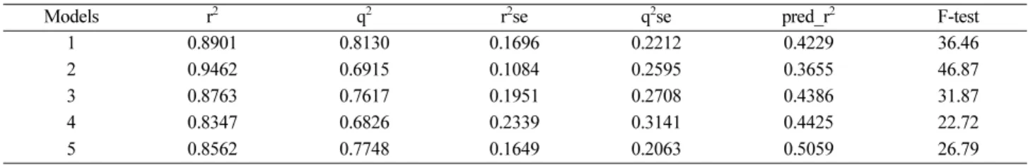
The selection of the best model is based on the values of r2 (squared correlation coefficient), q2 (cross-validated corre- lation coefficient), pred_r2 (predicted correlation coefficient for the external test set), F (Fisher ratio) reflects the ratio of the variance explained by the model and the variance due to the error in the regression. High values of the F–test indicate that the model is statistically significant. r2se, q2se and pred_r2se are the standard errors terms for r2, q2 and pred_r2 respectively. The statistically significant 2D-QSAR model is shown as follows.
Model-1 (Test set: 10, 13, 18, 7, 8, 9)
pIC50 = −0.2392 (T_2_N_1) + 0.2570 (SsCH3count) + 2.8148 Statistics:
[n = 12; Degree of freedom = 9; r2 = 0.8901; q2 = 0.8130;
F test = 36.4635; r2se = 0.1696;q2se = 0.2212; pred_r2 = 0.4229; pred_r2se = 0.4606]
Model-2 (Test size: 1, 13, 14, 15, 6, 8)
pIC50=−0.4102(T_N_S_3)− 0.5910 (T_N_CL_6)− 0.1347 (SaaaC count) + 1.9130
Statistics:
[n = 12; Degree of freedom = 8; r2 = 0.9462; q2 = 0.6915, F test = 46.8763; r2se = 0.1084; q2se = 0.2595; pred_r2 = 0.3655; pred_r2se = 0.5573]
In the above QSAR equations, n is the number of mol- ecules (Training set) used to derive the QSAR model, r2 is the squared correlation coefficient, q2 is the cross-vali- dated correlation coefficient, pred_r2 is the predicted cor- relation coefficient for the external test set, F is the Fisher ratio, reflects the ratio of the variance explained by the model and the variance due to the error in the regression.
High values of the F-test indicate that the model is sta- tistically significant. r2se, q2se and pred_r2se are the stan- dard errors terms for r2, q2 and pred_r2 (smaller is better).
Table 3. Statistical evaluation of 2D-QSAR models
Models r2 q2 r2se q2se pred_r2 F-test
1 0.8901 0.8130 0.1696 0.2212 0.4229 36.46
2 0.9462 0.6915 0.1084 0.2595 0.3655 46.87
3 0.8763 0.7617 0.1951 0.2708 0.4386 31.87
4 0.8347 0.6826 0.2339 0.3141 0.4425 22.72
5 0.8562 0.7748 0.1649 0.2063 0.5059 26.79
Interpretation of the Models Model-1
From equation, model-1 explains 89.01% (r2 = 0.8901) of the total variance in the training set as well as it has internal (q2) and external (pred_r2) predictive ability of 81.30% and 42.29% respectively. The F-test shows the statistical significance of 99.99% of the model which means
that probability of failure of the model is 1 in 10000. In addition, the randomization test shows confidence of 99.9999 (Alpha Rand Pred R^2 = 0.00000) that the generated model is not random and hence chosen as the QSAR model.
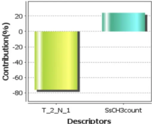
From QSAR model-1, negative coefficient value of T_2_N_1 [count of number of double bonded atoms (i.e., any double bonded atom, T_2) separated from nitrogen atom by sin- gle bonds] on the biological activity indicated that lower values leads to good inhibitory activity while higher value leads to reduced inhibitory activity while positive coef- ficient value of SsCH3count[the total number of CH3 group connected with single bond] on the inhibitory activity indicated that higher value leads to better inhibitory activity whereas lower value leads to decrease inhibitory activity.
Contribution chart for model-1 is represented in Fig. 3 reveals that the descriptors SsCH3count, contributing 25.70%
respectively. Another descriptors T_2_N_1 is contribut- ing inversely 23.92% respectively to biological activity.
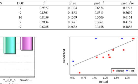
Data fitness plot for model-1 is shown in Fig. 4. The plot of observed vs predicted activity provides an idea about how well the model was trained and how well it predicts the activity of external test set.
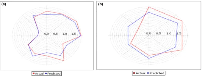
The graph of observed vs predicted activity of training and test sets for model-1 is shown in Figs. 5(a) and 5(b), it reveals that the model is able to predict the activity of training set quite well as well as external test set, provid- ing Confidence of model. Result of the observed and predicted inhibitory activity for the training and test compounds for the Model-1 is shown in Table 5.
From equation, Model-2 explains 94.62% (r2 = 0.9462) of the total variance in the training set as well as it has internal (q2) and external (pred_r2) predictive ability of 69.15% and 36.55% respectively. From QSAR model-2, it Figure 3. Plot of contribution chart for 2D-QSAR model-1.
Figure 4. Data fitness plot for 2D-QSAR model-1.
Figure 5. (a) Plot of observed versus predicted activity of 2D-QSAR model-1 (training set), (b) Plot of observed versus predicted activity of 2D-QSAR model-1 (test set).
was observed that Negative coefficient value of T_2_N_0 [count of number of double bonded atoms (i.e., any double bonded atom, T_2) separated from carbon atom], T_N_CL_6 [count of number of nitrogen atoms (single, double or tri- ple bonded) separated from any other chlorine atom (sin- gle or double or triple bonded) by 6 bonds in a molecule and SaaaCcount (total number of carbon connected with three aromatic bonds) on the biological activity indicated that lower values leads to good inhibitory activity while higher value leads to reduced inhibitory activity.
Contribution chart for model-2 is represented in Fig. 6,
it reveals that the descriptors T_2_N_0, T_N_CL_6, SaaaC- count contributing 41.02%, 59.10% and 13.47% respectively.
Data fitness plot for model-2 is shown in Fig. 7; the plot of observed vs predicted activity provides an idea about how well the model was trained and how well it predicts the activity of external test set.
The graph of observed vs predicted activity of training and test sets for model-2 is shown in Figs. 8(a) and 8(b), reveals that the model is able to predict the activity of training set quite well as well as external test set, provid- ing confidence of model. Result of the observed and predicted Figure 6. Plot of contribution chart for 2D QSAR model-2. Figure 7. Data fitness plot for 2D QSAR model-2.
Table 4. Statistical evaluation of 3D-QSAR models
Models kNN DOF q2 q2_se pred_r2 pred_r2se
1 2 7 0.9372 0.1304 0.6574 0.2777
2 2 9 0.8561 0.1863 0.5311 0.3699
3 2 10 0.8059 0.1569 0.3606 0.6174
4 2 9 0.9134 0.1471 0.3861 0.4158
5 2 9 0.6788 0.2632 0.3458 0.4888
Figure 8. (a) Plot of observed versus predicted activity of 2D-QSAR model-2 (training set), (b) Plot of observed versus predicted activ- ity of 2D-QSAR model-2 (test set).
inhibitory activity for the training and test compounds for the Model-2 is shown in Table 5.
3D-QSAR Model
kNN-MFA samples the steric and electrostatic fields surrounding a set of ligands and constructs 3D-QSAR mod- els by correlating these 3D fields with the corresponding biological activities. The statistical significant 3D-QSAR models Table 4.
The selection of the best model is based on the values of q2 (internal predictive ability of the model) and that of pred_r2 (the ability of the model to predict the activity of external test set). The statistical significant 3D-QSAR models for pIC50 (model-1) and pIC50 (model-2) are given below.
Model-1(3D)
pIC50=−S_2012(−0.0792, −0.0467) − S_2567(−0.0566,
−0.0152) − S_1620(−0.0789, −0.0441) + E_3168(0.0857, 0.0773)
Statistics:
[kNN = 2; n = 12; Degree of freedom = 7; q2 = 0.9372;
q2_se = 0.1304; pred_r2 = 0.6574; pred_r2se = 0.2777]
The model 1 explains values of k (2), q2 (0.9372), pred_r2 (0.6574), q2_se (0.1304), and pred_r2 se (0.2777) prove that QSAR equation so obtained is statistically significant
and shows the predictive power of the model is 93.72%
(internal validation). Table 5 represents the predicted inhibi- tory activity by the model-1 for training and test set.
The data fitness plot for model-1 is shown in Fig. 9. The plot of observed vs. predicted activity provides an idea about how well the model was trained and how well it pre- dicts the activity of the external test set.
From Figs. 10(a) and 10(b) it can be seen that the model is able to predict the activity of the training set quiet well as well as external test set, providing confidence of the model.
Result plot in which 3D-alignment of molecules with the important steric and electrostatic points contributing in the model-3 with ranges of values shown in the paren- thesis represented in Fig. 11. It shows the relative position and ranges of the corresponding important steric and elec- Figure 9. Data fitness plot for 3D-QSAR model-1.
Table 5. Actual and predicted activities for 18 compounds based on the best 2D/3D-QSAR models Compd. pIC50 2D-QSAR (model-1)
Predicted
3D-QSAR (model-1(3D)) Predicted
2D-QSAR (model-2) Predicted
3D-QSAR (model-2(3D)) Predicted
1 1.629 1.6365 1.8935 1.9129 1.1832
2 1.049 1.1581 1.8934 1.2335 1.5286
3 1.336 1.1581 1.8935 1.2335 1.5288
4 1.350 1.4152 1.8935 1.2335 1.5288
5 1.199 1.1581 1.4752 1.2335 1.5287
6 0.505 0.4583 1.8935 1.0926 1.5287
7 0.653 0.2191 1.9032 0.6824 1.5272
8 0.505 0.9367 1.9032 1.0926 1.5273
9 1.427 1.3973 1.9032 1.5028 1.5273
10 1.667 0.9367 1.8934 1.5028 1.5287
11 1.884 1.8936 1.4866 1.9129 1.5287
12 1.903 1.8936 1.8935 1.9129 1.5287
13 1.903 1.6722 1.8934 1.9129 1.5287
14 1.029 1.3973 1.8935 1.9129 1.5284
15 1.903 1.6365 0.5738 1.9129 1.5287
16 1.903 1.8936 1.8934 1.9129 1.5288
17 1.903 1.8936 1.8934 1.9129 1.5287
18 1.322 1.6365 1.6170 1.3222 1.5288
trostatic fields in the model provides guideline for new molecule design as follows.
(a) Electrostatic field, E_3168 (0.0857, 0.0773) has pos- itive range indicates that positive electrostatic potential is favorable for increase in the activity and hence less elec- tronegative substituent group is preferred in that region.
(b) Steric filed, S_2012 (−0.0792, −0.0467) has negative range indicates that negative steric potential is favorable for increase in the activity and hence less bulky substit- uent group is preferred in that region.
(c) Steric filed, S_2567 (−0.0566, −0.0152) also has neg- ative range indicates that negative steric potential is favor- able for increase in the activity and hence less bulky substituent group is preferred in that region.
(d) Steric filed, S_1620 (−0.0789, −0.0773) also has neg- ative range indicates that negative steric potential is favorable for increase in the activity and hence less bulky substit- uent group is preferred in that region.
Model-2(3D)
pIC50=−E_1712(−0.9546, −0.7371)+S_1633(0.1019, 0.1084)
Statistics:
[kNN = 2; n = 12; Degree of freedom = 9; q2= 0.8561;
q2_se = 0.1863; pred_r2 = 0.5311; pred_r2se = 0.3699]
In model 2(3D), values of kNN (2), q2 (0.8561), pred_r2 (0.5311), q2se (0.1863), and pred_r2se (0.3699) prove that QSAR equation so obtained is statistically significant and shows the predictive power of the model is 85.61% (inter- nal validation). Table 5 represents the predicted inhibitory activity by the model-2 (3D) for training and test set.
The data fitness plot for model-2(3D) is shown in Fig.
12. The plot of observed vs predicted activity provides an idea about how well the model was trained and how well it predicts the activity of the external test set.
From Figs. 13(a) and 13(b) it can be seen that the model is able to predict the activity of the training set quiet well as well as external test set, providing confidence of the model.
Result plot in which 3D-alignment of molecules with the important steric and electrostatic points contributing in the model with ranges of values shown in the paren- thesis represented in Fig. 14. It shows the relative position Figure 10. (a) Plot of observed versus predicted activity of 3D-QSAR model-1 (training set), (b) Plot of observed versus predicted activ- ity of 3D-QSAR model-1 (test set).
Figure 11. Plot of contribution chart for 3D QSAR model-1.
Figure 12. Data fitness plot for 3D QSAR model-2.
and ranges of the corresponding important steric and elec- trostatic fields in the model provides guideline for new molecule design as follows.
(a) Electrostatic field, E_1712 (−0.9546, −0.7371) has negative range indicates that negative electrostatic poten- tial is favorable for increase in the activity and hence more electronegative substituent group is preferred in that region.
(b) Steric field, S_1633 (0.1009, 0.1084) has positive range indicates that positive steric potential is favorable for increase in the activity and hence more bulky substit- uent group is preferred in that region.
CONCLUSION
Statistically significant 2D/3D-QSAR models were gen- erated with the purpose of deriving structural requirements for the inhibitory activities of some imidazole-(benz)azole derivatives against breast MCF-7 cell lines. The validation of 2D-QSAR models was done by the cross-validation test,
randomization tests and external test set prediction. The best 2D-QSAR models indicate that the descriptors of SsCH3count, T_2_N_1 influenced the inhibition activity.
kNN-MFA investigated the substitutional requirements for the receptor-drug interaction and constructed the best 3D- QSAR models by Multiple Linear Regression method, providing useful information in characterization and dif- ferentiation of their binding sites. In conclusion, the infor- mation provided by the robust 2D/3D-QSAR models use for the design of new molecules (Table 6) and hence, this Figure 13. (a) Plot of observed versus predicted activity for 3D-QSAR model-2 (training), (b) Plot of observed versus predicted activity of 3D QSAR model-2 (test set).
Figure 14. Plot of contribution chart for 3D-QSAR model-2.
Table 6. Structure and predicted activity of newly designed com- pounds
Compd. R Predicted activity
(pIC50)*
Antilog of pIC50
1 1.89361 78.2726
2 1.89361 78.2726
3 1.91144 81.553
4 1.89361 78.2726
5 2.40768 255.6701
6 2.15064 141.4621
7 2.40768 255.6701
*Increased predicted activity.
method is expected to provide a good alternative for the drug design.
Acknowledgments. The authors are thankful to V-Life Sciences Technologies Private Limited, 1 Akshay, 50 Anand Park, Aundh, Pune, India for providing trial version of the software. And the publication cost of this paper was sup- ported by the Korean Chemical Society.
REFERENCES
1. Krikas, G.; Schulpis, K.; Reclos, G.; Kokotos, G. Clin.
Biochem. 1998, 31, 405.
2. Waring, M.; Bailly, C. Gene 1994, 149, 69.
3. Rehn, C.; Pindur, U. Monatsh. Chem. 1996, 127, 631.
4. Baginski, M.; Fogolari, F.; Briggs, J. J. Mol. Biol. 1997, 274, 253.
5. Shui, X.; et al. Curr. Med. Chem. 2000, 7, 59.
6. Neidle, S. In Cancer Drug Desing and Discovery, 2nd Ed.; Elsevier Inc.: U.S.A., 2008, p 132.
7. Moore, M.; Hunter, W.; Langlis-D’Estaintot, B.; Kennard, O.
J. Mol. Bio. 1989, 206, 693.
8. Pindur, U.; Haber, M.; Sattler, K. J. Chem. Educ. 1993, 70, 263.
9. Zhigang, L.; Qing, Y.; Xuhong, Q. Bioorg. Med. Chem.
Lett. 2005, 15, 3143.
10. Claiborne, C.; Liverton, N.; Nguyen, K. Tetrahedron Lett.
1998, 39, 8939.
11. Cui, B.; Zheng, B.; He, K.; Zheng, Q. J. Nat. Prod. 2003, 66, 1101.
12. Fazeny-Dorner, B.; Veitl, M.; Wenzel, C.; Piribauer, M.;
Rossler, K.; Dieckmann, K.; Ungersbock, K.; Marosi, C.
Anticancer Drugs. 2003, 14, 437.
13. Haluska, P.; Dy, G.; A. Adjei, A. Eur. J. cancer. 2008, 38, 1685.
14. Kotteas, E.; Alamara, C.; Kiagia, M.; Pantazopoulos, K.;
Oufas, A.; Provata, A.; Chapidou, A.; Syrigos, K. N. Antican- cer Res. 2008, 28, 529.
15. Perez-ruixo, J.; Piotrovskij, V.; Zhang, S.; Hayes, S.; DePorre, P.; Zannikos, P. Br. J. Clin, Pharmacol. 2006, 62, 81.
16. Krezel, I. Farmaco 1998, 53, 342.
17. Kumar, D.; Jacob, M. R.; Reynolds, M. B.; Kerwin, S. M.
Bioorg. Med. Chem. 2002, 10, 3997.
18. Hose, C.; Hollingshead M.; Sausville E.; Monks A.; Mol.
Cancer Ther. 2003, 2, 1265.
19. Al-Masoudi, A.; Al-Soud, Y.; Al-Salihi, N.; Al-Masoudi, N. Chem. Hetetrocycl. Compd. 2006, 42, 1377.
20. Jackman, A.; Kimbell, R.; Aherne, G.; Brunton, L.; Jan- sen, G.; Stephens, T.; Smith, M.; Wardleworth, J.; Boyle, F. Clin. Cancer Res. 1997, 3, 911.
21. Nelson, J.; Rose, L.; Benneft, L. Cancer Res. 1977, 37, 182.
22. Martin, B.; Mann, J.; Sageot, A. J. Chem. Soc. Perkin Trans.
1, 1999, 2455.
23. Brian, B.; Andrew, M.; Hana, K.; Padmakumari, T.; Wil- liam, P.; Jack, C. Mol. Pharmacol. 1997, 52, 839.
24. Hansch, C.; Kurup, A.; Garg, R.; Gao, H. Chem. Rev. 2001, 101, 619.
25. Yusuf, O.; Ilhan, I.; Zerrin, I.; Gulsen, A. Eur. J. Med.
Chem. 2010, 45, 3320.
26. Golbraikh, A.; Tropsha, A. J. Comput. Aided Mol. Des.
2002, 16, 357.
27. VLifeMDS 4.2; Molecular Design Suite; Vlife Sciences Technologies Pvt. Ltd.: Pune, India, 2012. www.vlife- sciences.com
28. Gasteiger, J; Marsili, M. Tetrahedron. 1980, 36, 3219.
29. Ajmani, S.; Jhadav, K.; Kulkarni, S. A. J. Chem. Inf. Model.
2006, 46, 24.
![Table 1. Chemical structures of 2-substituted-N-[4-(1-methyl-4,5- 2-substituted-N-[4-(1-methyl-4,5-diphenyl-1H-imidazole-2-yl)phenyl] acetamide derivatives](https://thumb-ap.123doks.com/thumbv2/123dokinfo/5298934.154266/2.892.461.809.185.1049/chemical-structures-substituted-substituted-diphenyl-imidazole-acetamide-derivatives.webp)
![Figure 2. 3D view of aligned 2-substituted-N-[4-(1-methyl-4,5- 2-substituted-N-[4-(1-methyl-4,5-diphenyl-1H-imidazole-2-yl)phenyl] acetamide derivatives.](https://thumb-ap.123doks.com/thumbv2/123dokinfo/5298934.154266/4.892.493.775.826.1063/figure-aligned-substituted-substituted-diphenyl-imidazole-acetamide-derivatives.webp)