Experimental Study on the Unsteady Flow Characteristics for the Counter-Rotating Axial Flow Fan
L. S. Cho*, S. W. Lee*, J. S. Cho†
*Department of Mechanical Engineering, Hanyang University 17 Haengdang-Dong, Sungdong-Ku, Seoul 133-791, Korea
†School of Mechanical Engineering, Hanyang University 17 Haengdang-Dong, Sungdong-Ku, Seoul 133-791, Korea
and J. S. Kang‡
‡KHP Development Division, Korea Aerospace Research Institute 45 Eoeun-Dong, Yuseong-Gu, Daejeon 305-806, Korea
Keywords: Counter-Rotating Axial Flow Fan, Three-Dimensional Unsteady Flow, 45° Inclined Hot-Wire
Abstract
Counter-rotating axial flow fan(CRF) consists of two counter-rotating rotors without stator blades. CRF shows the complex flow characteristics of the three- dimensional, viscous, and unsteady flow fields.
For the understanding of the entire core flow in CRF, it is necessary to investigate the three- dimensional unsteady flow field between the rotors.
This information is also essential to improve the aerodynamic characteristics and to reduce the aerodynamic noise level and vibration characteristics of the CRF.
In this paper, experimental study on the three- dimensional unsteady flow of the CRF is performed at the design point (operating point). Flow fields in the CRF are measured at the cross-sectional planes of the upstream and downstream of each rotor using the 45°
inclined hot-wire. The phase-locked averaged hot-wire technique utilizes the inclined hot-wire, which rotates successively with 120 degree increments about its own axis.
Three-dimensional unsteady flow characteristics such as tip vortex, secondary flow and tip leakage flow in the CRF are shown in the form of the axial, radial and tangential velocity vector plot and velocity contour.
The phase-locked averaged velocity profiles of the CRF are analyzed by means of the stationary unsteady measurement technique.
At the mean radius of the front rotor inlet and the outlet, the phase-locked averaged velocity profiles show more the periodical flow characteristics than those of the hub region.
At the tip region of the CRF, the axial velocity is decreased due to the boundary layer effect of the fan casing and the tip vortex flow. The radial and the tangential velocity profiles show the most unstable and unsteady flow characteristics compared with other position of rotors. But, the phase-locked averaged velocity profiles of the downstream of the rear rotor show the aperiodic flow pattern due to the mixture of the front rotor wake period and the rear rotor rotational period.
* Professor, [email protected]
Introduction
Counter-rotating axial flow fan(CRF), which is a kind of two-stage axial-flow fan, has been a good solution for applications where high static pressure rise and volumetric flow rate are required[1]. CRF consists of two counter-rotating rotors, without stator blades[2]. Compared with commercial single-rotating axial flow fan, the CRF has higher performance characteristics and higher efficiency because the swirl velocity generated by the front rotor, which causes the energy loss, is recovered in the form of the static pressure by the rear rotor[3].
Counter-rotating systems[4] were developed at the National Aeronautics and Space Administration (NASA) in USA for the aircraft propulsion system because of its higher propulsion efficiency and lower specific fuel consumption, relatively.
The aerodynamic characteristics of the CRF have investigated by several researchers. Kodama et al.[5]
showed that the fluid dynamic characteristics of the CRF are superior to those of the two-stage axial flow fan. Shin et al.[6] investigated the rotor-rotor interaction of counter-rotating unducted fans.
The CRF shows the complex flow characteristics of the three-dimensional, viscous, and unsteady flow fields. Therefore, the aerodynamic noise level of the CRF is increased due to rotor-rotor interaction by the two rotors with opposite directional rotation[6].
For the understanding of the entire core flow in the CRF, it is necessary to investigate the three- dimensional unsteady flow field between two rotors.
This information is also essential to predict the aerodynamic and the acoustical characteristics of the CRF.
In this present paper, experimental study on the three-dimensional unsteady flow of the CRF is carried out at the design point(operating point). Flow fields in the CRF are measured at the cross-sectional planes of the upstream and downstream of each rotor using the 45° inclined hot-wire. The phase-locked averaged hot- wire technique utilizes the inclined hot-wire, which rotates successively with 120 degree increments about its own axis. Three-dimensional unsteady flow characteristics in the CRF are shown in the form of the axial, radial and tangential velocity vector plot and velocity contour.
Experimental Setup
The experimental apparatus, as shown in Fig. 1, was set up for the investigation of three-dimensional unsteady flow fields in the CRF. Its total length is 7,650mm and the diameter of the tested fan casing is 500mm.Test setups do not utilize an auxiliary fan and a duct system consists of the discharge duct only. A bell mouth, which is installed at the inlet of the tested fan, reduces the energy loss due to fluid friction and flow separation of the inlet flow. A conical damper is used to adjust the flow rate at the exit of the test duct.
The CRF consists of a front rotor and a rear rotor.
The two rotors rotate in opposite direction and are driven by two separate electric motors. The front rotor of the CRF has eight blades and the rear rotor has seven blades as shown in Fig. 2.
Dimensions of the front rotor and the rear rotor are shown in Table 1. The diameter of the rotor is 497mm, and the hub-tip ratio is 0.4. The front rotor blades show opposite twist distributions compared with rear rotors.
Figure 3 shows the cross-sectional blade shape for the front rotor and the rear rotor at the blade hub, the mid span and the tip of the CRF.
Velocity triangles of the CRF are shown in Fig. 4.
The stagger angle of the front rotor blade is 6 degree lower than the rear rotor because of the increment of the relative velocity due to the opposite rotational direction of the rear rotor compare with the front rotor.
Figure 5 shows characteristic curves of the CRF, which are based on the KS B 6311(Testing Methods for Turbo Fans and Blowers)[7]. Three-dimensional unsteady flow fields in the CRF are measured at the peak efficiency operating condition as shown in Table 2.
Fig. 1 Schematic diagram of the experimental setup, dimensions in mm
(a) Front rotor(NB=8) (b) Rear rotor(NB=7) Fig. 2 Front view of the front rotor and the rear rotor of the counter-rotating axial flow fan
Table 1 Specifications of the tested fan rotor blades Front rotor Rear rotor
Fan diameter 500 mm 500 mm
Tip diameter 497 mm 497 mm
Hub diameter 199 mm 199 mm
Airfoil Shape NACA65-series Camber angle 18 deg.
Max. Thickness 10 %(=12.825 mm) Stagger angle
at 0.75 radius 54.0 deg. 60.0 deg.
Solidity
at 0.75 radius 0.8 0.7
Number of blades 8 7
z(m)
θ(m)
-0.05 0 0.05 0.1 0.15 0.2 0.25
-0.06 -0.04 -0.02 0 0.02 0.04 0.06
hub mid tip
hub mid tip
Rear Rotor Front Rotor
Rotationaldirection Rotationaldirection
Fig. 3 Cross sectional blade shape of the counter- rotating axial flow fan
Fig. 4 Velocity triangles of the counter-rotating axial flow fan
Flow coefficient,φ Fanefficiency,η Pressurecoefficient,ψ Shaftpowercoefficient,λ
0 0.1 0.2 0.3 0.4 0.5
0 0.2 0.4 0.6 0.8 1
CRF(NB= 8× 7) ξFR=54°, ξRR=60°
ψλ η
Stalling onset
Peak efficiency
Fig. 5 Characteristic curves of the counter-rotating axial flow fan
7,650 1,650
6000
500
800
Motor Bell Mouth
Honeycomb
Dynamic Pressure Tap Damper Static Pressure Tap
Motor
Front Rotor Rear Rotor
Table 2 Peak efficiency operating conditions of the counter-rotating axial flow fan
Performance parameter Operating condition Total pressure rise(ΔPT) 27mmH2O
Volumetric flow rate(Q) 2.8m3/s Fan efficiency(η ) fan 83.6%
Rotational speed(N) 1750rpm Experimental Methods
Three-dimensional unsteady flow fields in the CRF are investigated using a single 45 degree inclined hot- wire sensor. Many investigators have used the single- sensor hot-wire system for the measurement of three- dimensional flow fields and Reynolds stresses. A single-sensor hot-wire measurement technique is developed by Whitfield, et al. [8] and Hirsh and Kool[9] has made attempts to extend these techniques to the measurement of turbulence intensities of the exit flow of a rotor.
Configuration of a inclined hot-wire probe
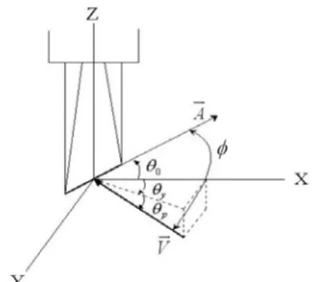
Configuration of a single 45 degree inclined hot- wire probe is shown in Fig. 6. The inclined angle of the hot-wire sensor is represented by the unit vector
urA
slanted at the probe angle θ to the 0 Xaxis. The probe coordinates X Y, and Z are fixed to the probe, the velocity vector is denoted by Vur. The probe yaw angle θ changes by the turning angle while the pitch y angle θ remains constant as the probe is rotated P about its axis. The sensor yaw angle φ can be expressed in terms of the angles θ ,0 θ , and P θ as y follows.
0 0
cosφ=cosθ ⋅cosθp⋅cosθy+sinθ ⋅sinθp (1) The relation between the velocity vector Vur and the hot-wire sensor is found in Reference[9].
Fig. 6 Schematic diagram of the single 45° inclined hot-wire probe
Calibration of a slanted hot-wire probe
The velocity calibration of the single 45 degree slanted hot-wire probe was carried out with the sensor yaw angle θ equals to 90 degree by the method of y Grand and Kool[10] in wind tunnel(0≤ ≤V 60m/s).
The turbulence level of the open type wind tunnel was 0.13 percent. The relation between the bridge voltage( E ) and the effective cooling velocity(Ve) is expressed by the King’s law.
E2 = +A B Ven (2) where the three coefficients A , B and n are determined from a velocity calibration data obtained using the hot-wire sensor normal to the flow.
Probe-angle calibrations were done at fixed values of velocity and angle between probe axis and velocity vector. Probe-angle calibrations, on the other hand, were carried out a large range of probe angles (− ≤90 θy≤ + degree). During these calibrations the 90 probe was always rotated in the same manner.
The ratio of effective cooling velocity Ve and actual velocity V is expressed in terms of the angles θ , 0 θ , P and θ as follows[10]. y
e cos V
V = ψ (3)
2 2 0
1
sin A cos pcos y A tan sin p
A
ψ = θ ⎛⎜⎝θ ⎞⎟⎠+ θ θ (4) where ψ is a parameter in experimental probe angle calibration law.
The velocity calibration results of the 45° slanted hot-wire probe are fitted by the nonlinear curve fitting as shown in Fig. 7. Figure 8 shows the probe angle calibration curves. Relation between yaw angle and velocity was used because the probe-angle calibration curves were not always symmetric. The coefficients of the equation (2) and equation (4) were determined by the least square fitting of the effective cooling velocity data.
Fig. 7 Velocity calibration results of the 45° slanted hot-wire probe
Fig. 8 Probe yaw angle calibration results of the 45°
slanted hot-wire probe
Yaw angle(degree)
Ve/V
-90 -60 -30 0 30 60 90
0.5 0.6 0.7 0.8 0.9 1
1.1 Experimental results Nonlinear curve fitting results Data: Data1-B
Model: user3 Chi2= 0.00023 A1 1.01427 ± 0.01185 A2 0.83797 ± 0.00341
Velocity(m/s)
Voltage(V)
0 10 20 30 40 50 60
2 2.5 3 3.5
4 Experimental results Nonlinear curve fitting results
Data: Data1-B Model: user1 Chi2= 0.00002 A 3.27836 ± 0.01587 B 1.55725 ± 0.01248 n 0.45801 ± 0.00184
Measurement location and technique
Three-dimensional unsteady flow fields in the CRF were measured at cross-sectional planes of seven axial stations (upstream of the front rotor, between two rotors, and downstream of the rear rotor).
Figure 9 shows the schematic drawings of the CRF model and the single 45° inclined hot-wire probe measurement locations. At the peak efficiency operating point of the CRF, three-dimensional unsteady flow fields were measured at 23 points(r r/ tip=0.4 to 1.0) for the radial direction. Also, circumferential flow fields in the CRF are investigated at 345 points (0.52 degree interval) for 4 blade passage of the front rotor(3.5 blade passage of the rear rotor).
The stationary hot-wire technique utilizes a single sensor, which rotates successively with 120 degree increments about its own axis. By placing the probe at different positions characterized by θ , y θy+ , and θ1
y 2
θ +θ where θ and 1 θ are the amounts of turning, 2 a set of three equations can be derived as follows.
2
2
2
2 2
1 1
2 2
2 2
2 2
3 3
(1 sin ) (1 sin ) (1 sin )
e e
e
V V
V V
V V
ψ ψ ψ
⎧ = −
⎪⎪ = −
⎨⎪
= −
⎪⎩
(5)
1 2 2 0
1
1
2 2 2 0
1
2
3 2 2 0
1
sin cos cos tan sin
sin cos cos tan sin
sin cos cos tan sin
y
p p
y
p p
y
p p
A A
A
A A
A
A A
A
ψ θ θ θ θ
θ θ
ψ θ θ θ
θ θ
ψ θ θ θ
⎧ = ⎛⎜ ⎞⎟+
⎪ ⎝ ⎠
⎪⎪ +
⎪ = ⎛ ⎞+
⎨ ⎜⎝ ⎟⎠
⎪⎪ = ⎛ + ⎞+
⎪ ⎜ ⎟
⎪ ⎝ ⎠
⎩
(6)
Since the effective cooling velocities are known and six unknown variables(ψ , 1 ψ ,2 ψ , 3 θ ,P θ , and V ) y remain, and the six nonlinear equations(eq.(5, 6)) could be solved simultaneously by using the Newton- Raphson numerical method.
Non-dimensional axial distance(z/rtip) Non-dimensionalradialdistance(r/rtip)
-0.2 0 0.2 0.4 0.6 0.8 1
0.3 0.4 0.5 0.6 0.7 0.8 0.9 1 1.1
Rear rotor Front rotor
(z/rtip= 0.436)
(z/rtip= -0.02) (z/rtip= 0.88)
(z/rtip= 0.332)
(z/rtip= 0.384) (z/rtip= 0.488) (z/rtip= 0.54)
Station 1 Station 2 Station 3
Fig. 9 Hot-wire probe measuring points for three- dimensional unsteady flow fields of the counter- rotating axial flow fan
Data Acquisition and Data Reduction
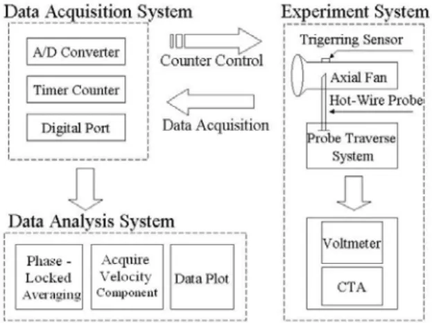
The data acquisition process of the hot-wire probe is shown in Fig. 10. The raw signal from the bridge output includes the random data as well as the phase information. In this technique, the hot-wire signal is triggered by a revolution frequency pulse in successive wave forms and are then averaged with one another so that only velocity components repeated every rotor revolution can be obtained. With the probe sensor positioned at 90 degree(normal to the rotor axis), the probe was rotated with the three different yaw angles. A rotor 1/rev signal was fed into the stop trigger of the A/D converter module. The A/D converter speed was set at 100kHz and a 2,000 sample memory was allocated for the sample memory module operating in a post trigger. The sampling data were taken for 4 blade passage of the front rotor (3.5 blade passages of the rear rotor), at each probe angle position and transferred to the computer. The instantaneous voltage data were converted into the effective level using the velocity calibration information.
The sampling data were phase-locked averaged to remove the random component. Figure 11 shows phase-locked averaging process for the output voltage signal of the 45° slanted hot-wire probe. At each of 250 phase-lock positions 100sets of data were taken and averaged.
Fig. 10 Schematic diagram of instrumentation for the 45° slanted hot-wire
Fig. 11 Phase-locked averaging process for the output voltage signal of the 45° slanted hot-wire probe
Measurement accuracy
For the analysis of the measurement accuracy of three-dimensional unsteady flow fields in the CRF, calibration data were compared with converting data obtained from the nonlinear equations.
Figure 12 shows the yaw angle error between the real probe yaw angle and the computed probe yaw angle by nonlinear equations. Maximum error of the probe yaw angle was about 5 degree. Fig. 13 shows the error of the axial velocity magnitude between the real velocity profile and the computed velocity profile by nonlinear equation. Maximum error of the velocity profile was about 7%. When the yaw angle of the hot- wire probe is 35 degree∼ degree to the real fluid 50 flow, the real flow fields are relatively accurate.
Hot-wire probe yaw angle (degree)
Error(degree)
0 20 40 60 80
0 2 4 6 8 10
< Yaw angle error >
V=20m/s
Fig. 12 Probe yaw angle measurement accuracy
Fig. 13 Velocity magnitude measurement accuracy Results and Discussion
The three-dimensional unsteady flow fields of the CRF is showed in the form of phase-locked averaged velocity profiles and the velocity contours, which are measured at seven axial stations(upstream of the front rotor, between the rotors and downstream of the rear rotor) by the single 45 degree slanted hot-wire sensor.
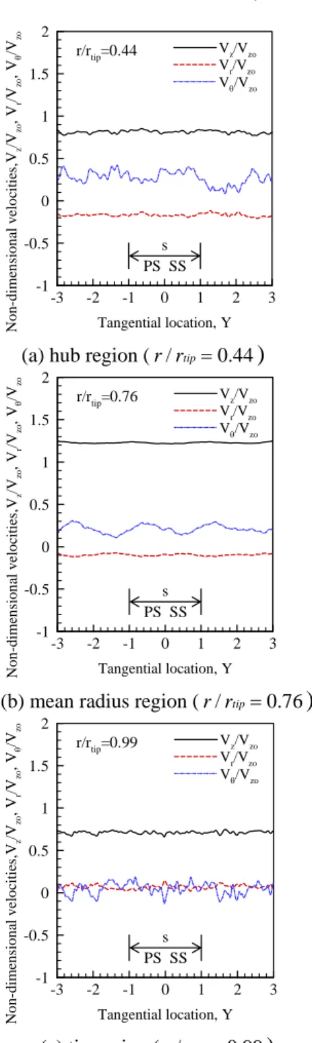
Figure 14 shows phase-locked averaged velocity profiles at station 1(upstream of the front rotor) of the CRF. Velocity profiles are normalized by the averaged axial velocity Vz0 in the CRF. Also, rotor blade passage is normalized by the parameter Y , which are the interval of corresponds to 0.5 blade passage for the front rotor and the rear rotor.
Y 2r s
= θ (7)
Here r is the measuring location in the radial direction, θ is the measuring position in the tangential direction, and s is the blade spacing. If the interval of the non-dimensional parameter Y is 2, Y means 1 blade passage. The measuring velocity profile data were 86 points for 4.3ms per 1 blade passage of the front rotor. Rear rotor is 98 data points for 4.9ms per 1 blade passage.
Fig. 14(a) shows the phase-locked averaged velocity profiles for 3 blade passages at the hub region of the front rotor inlet. The axial velocity is decreased due
Tangential location, Y Non-dimensionalvelocities,Vz/Vzo,Vr/Vzo,Vθ/Vzo
-3 -2 -1 0 1 2 3
-1 -0.5 0 0.5 1 1.5 2
Vz/Vzo r/rtip=0.44
s PS SS
Vr/Vzo Vθ/Vzo
(a) hub region (r r/ tip=0.44
)
Tangential location, Y Non-dimensionalvelocities,Vz/Vzo,Vr/Vzo,Vθ/Vzo
-3 -2 -1 0 1 2 3
-1 -0.5 0 0.5 1 1.5 2
Vz/Vzo r/rtip=0.76
s PS SS
Vr/Vzo Vθ/Vzo
(b) mean radius region (r r/ tip=0.76
)
Tangential location, Y Non-dimensionalvelocities,Vz/Vzo,Vr/Vzo,Vθ/Vzo
-3 -2 -1 0 1 2 3
-1 -0.5 0 0.5 1 1.5 2
Vz/Vzo r/rtip=0.99
s PS SS
Vr/Vzo Vθ/Vzo
(c) tip region (r r/ tip=0.99
)
Fig. 14 Phase-locked averaged velocity profiles at station 1(z r/ tip= −0.02) in the counter-rotating axial flow fan (Vzo=16.6m/s)
Hot-wire probe yaw angle (degree)
Error(%)
0 20 40 60 80
0 2 4 6 8 10
< Velocity error >
V=20m/s
to the flow separation by the installation of the front driving motor and the hub vortex by the rotation of the front rotor compared with mean axial velocity Vz0. The radial velocity is increased in the hub direction (negative direction) due to the flow contraction by the suction effect of the front rotor blade. The tangential velocity is increased at the front of the blade leading edge due to the blockage effect of the front rotor blade. At the whole, the phase-locked averaged velocity profiles showed the unstable flow characteristics such as the flow separation and the hub vortex.
Fig. 14(b) shows the phase-locked averaged velocity profiles at the mean radius of the front rotor inlet. The axial, the radial and the tangential velocity profiles at the mean radius show more periodical flow characteristics than those at the hub region. The axial velocity is more increased than the mean axial velocity Vz0. The radial and the tangential velocity profiles at the mean radius are similar to flow patterns compared with those of the hub region.
Fig. 14(c) shows the phase-locked averaged velocity profiles at the tip region of the front rotor inlet. The axial velocity is decreased due to the boundary layer effect of the fan casing and the tip leakage flow. The radial and the tangential velocity profiles show the most unstable and unsteady flow characteristics compare with other position of the fan inlet.
Figure 15 shows phase-locked averaged velocity profiles at station 2-3(between the rotors) of the CRF.
Fig. 15(a) shows the phase-locked averaged velocity profiles at the hub region of the between the rotors. The axial velocity is decreased due to the flow separation and the boundary layer effect of the front rotor hub and the front motor. The radial velocity is not appeared in the similar manner other axial flow type turbomachinery. The tangential velocity is increased due to the rotation of the front rotor blade compared with the front rotor inlet. At the whole, the phase-locked averaged velocity profiles of the front rotor outlet are periodically decreased due to the blockage effect at the trailing edge of the front rotor blade.
Fig. 15(b) shows the phase-locked averaged velocity profiles at the mean radius of the front rotor outlet.
The axial velocity is more increased than that of the front rotor inlet due to flow contraction effect. The radial velocity profile is hardly appeared. But, the tangential velocity is increased in the similar manner to the result of the free vortex design condition afterward the trailing edge of the front rotor blade. Fig.
15(c) shows the phase-locked averaged velocity profiles at the tip region of the front rotor outlet. The axial velocity is decreased in the form of the reverse flow by the tip leakage flow and the tip vortex. The tangential velocity profile is decreased and is different from the result of the free vortex design condition. At the blade passage between the suction side(upper surface) and the pressure side(lower surface) of the
rotor blade, the tangential velocity profile is decreased in the reverse direction by the tip vortex.
Figure 16 shows phase-locked averaged velocity profiles at station 3(downstream of the rear rotor) of the CRF. Fig. 16(a) shows the phase-locked averaged velocity profiles at the hub region of the rear rotor outlet. The axial velocity is decreased in the reverse direction by the hub vortex and the flow separation of the rear rotor. The tangential velocity is increased by the hub vortex due to the rotation of the rear rotor. Fig.
16(b) shows the phase-locked averaged velocity profiles at the mean radius of the rear rotor outlet. The axial velocity is more increased than that of the front rotor inlet and the outlet due to increment of the flow
Tangential location, Y Non-dimensionalvelocities,Vz/Vzo,Vr/Vzo,Vθ/Vzo
-3 -2 -1 0 1 2 3
-1 -0.5 0 0.5 1 1.5 2
Vz/Vzo r/rtip=0.44
s PS SS
Vr/Vzo Vθ/Vzo
(a) hub region (r r/ tip=0.44
)
Tangential location, Y Non-dimensionalvelocities,Vz/Vzo,Vr/Vzo,Vθ/Vzo
-3 -2 -1 0 1 2 3
-1 -0.5 0 0.5 1 1.5 2
Vz/Vzo r/rtip=0.76
s PS SS
Vr/Vzo Vθ/Vzo
(b) mean radius region (r r/ tip=0.76
)
Tangential location, Y Non-dimensionalvelocities,Vz/Vzo,Vr/Vzo,Vθ/Vzo
-3 -2 -1 0 1 2 3
-1 -0.5 0 0.5 1 1.5 2
Vz/Vzo r/rtip=0.99
s PS SS
Vr/Vzo Vθ/Vzo
(c) tip region (r r/ tip=0.99
)
Fig. 15 Phase-locked averaged velocity profiles at station 2(z r/ tip=0.436) in the counter-rotating axial
flow fan (Vzo=16.6m/s)
contraction effect. The tangential velocity is remained because the static pressure recovery for the swirl velocity component by the rotation of the front rotor is not completed. Fig. 16(c) shows the phase-locked averaged velocity profiles at the tip region of the rear rotor outlet. The axial velocity is increased due to the minimum of the leakage flow and the mixture of the front rotor and the rear rotor tip vortex. The tangential velocity is appeared in the rotational direction of the rear rotor due to the leakage flow not tip vortex of the rear rotor.
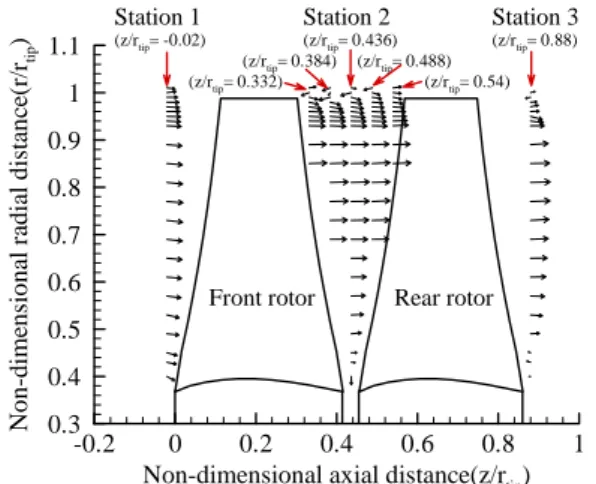
Figure 17 shows the circumferential averaged axial and radial velocity vectors for the through-flow fields
Tangential location, Y Non-dimensionalvelocities,Vz/Vzo,Vr/Vzo,Vθ/Vzo
-3 -2 -1 0 1 2 3
-1 -0.5 0 0.5 1 1.5 2
Vz/Vzo r/rtip=0.44
s PS SS
Vr/Vzo Vθ/Vzo
(a) hub region (r r/ tip=0.44
)
Tangential location, Y Non-dimensionalvelocities,Vz/Vzo,Vr/Vzo,Vθ/Vzo
-3 -2 -1 0 1 2 3
-1 -0.5 0 0.5 1 1.5 2
Vz/Vzo r/rtip=0.76
s PS SS
Vr/Vzo Vθ/Vzo
(b) mean radius region (r r/ tip=0.76
)
Tangential location, Y Non-dimensionalvelocities,Vz/Vzo,Vr/Vzo,Vθ/Vzo
-3 -2 -1 0 1 2 3
-1 -0.5 0 0.5 1 1.5 2
Vz/Vzo r/rtip=0.99
s PS SS
Vr/Vzo Vθ/Vzo
(c) tip region (r r/ tip=0.99
)
Fig. 16 Phase-locked averaged velocity profiles at station 3(z r/ tip=0.88) in the counter-rotating axial flow fan (Vzo=16.6m/s)
Non-dimensional axial distance(z/rtip) Non-dimensionalradialdistance(r/rtip)
-0.2 0 0.2 0.4 0.6 0.8 1
0.3 0.4 0.5 0.6 0.7 0.8 0.9 1 1.1
Rear rotor Front rotor
(z/rtip= 0.436)
(z/rtip= -0.02) (z/rtip= 0.88)
(z/rtip= 0.332)
(z/rtip= 0.384) (z/rtip= 0.488) (z/rtip= 0.54)
Station 1 Station 2 Station 3
Fig. 17 Circumferential averaged axial and radial velocity vectors of the counter-rotating axial flow fan in the CRF. As shown in Fig. 17, fan inlet flow field of the ahead the front rotor(station 1) is relatively uniform except decrement of the axial velocity due to the boundary layer effect of the fan casing and the tip leakage flow. At the tip region of the between the rotors(station 2), axial velocity is decreased from
/ tip 0.332
z r = to z r/ tip=0.488 of the axial direction due to the tip vortex of the front rotor. At the whole, axial velocity is gradually increased at the mean radius due to the flow contraction effect. At the hub region, axial velocity is gradually decreased and the radial velocity is increased due to the flow separation and the hub vortex.
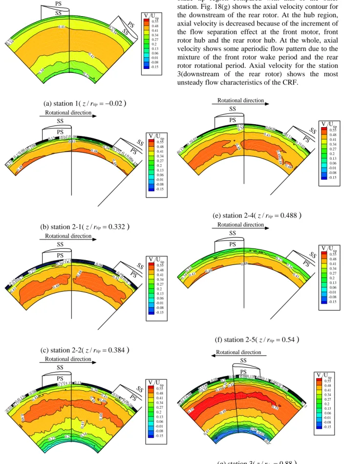
Figure 18 shows the axial velocity contours, which are normalized by the rotational speed(Utip
),
for the through-flow fields of the CRF. Axial velocity contours show the periodic flow characteristics by the blockage effect of the front rotor and the rear rotor blades. Fig. 18(a) shows the axial velocity contour for the cross flow pattern at the upstream of the front rotor.Axial velocity is increased at the mean radius due to flow contraction effect as shown in Fig. 14(b). At the blade tip region, the axial velocity is decreased because of the boundary layer effect by the fan casing.
Also, the axial velocity is decreased due to the flow separation by the front motor at the hub region. Fig.
18(b) shows the axial velocity contour at the downstream of the front rotor. At the blade tip region, the axial velocity is decreased due to the boundary layer effect by the fan casing and the blade tip vortex.
Also, axial velocity shows the reverse flow pattern in the axial direction by the tip vortex. This flow pattern is shown to the station 2-4(z r/ tip=0.488).
As shown in Fig. 18(c), the axial velocity of the blade tip region shows the reverse flow due to the tip vortex after the trailing edge of the front rotor.
Fig. 18(d) shows the axial velocity contour between the rotors. Axial velocity is increased due to the flow contraction at the mean radius compare with that of the station 1(before the front rotor).
As shown in Fig. 18(e), flow pattern of the axial velocity is similar to station 2-2(z r/ tip=0.332) but
the effect of the tip vortex by the rotation of the front rotor is decreased.
0.27 0.27
0.27
0.34 0.34
0.34 0.41
0.41
0.55 0.48 0.41 0.34 0.27 0.2 0.13 0.06 -0.01 -0.08 -0.15
SS PS
Vz/Utip SSPS
Rotational direction
(a) station 1(z r/ tip= −0.02
)
-0.15
-0.15-0.15 -0.15
-0.08
-0.08 -0.08
-0.01 -0.01
0.06 0.06 0.06
0.13 0.13
0.13
0.2 0.270.2
0.27
0.34 0.41
0.48 0.48
0.48
0.55 0.48 0.41 0.34 0.27 0.2 0.13 0.06 -0.01 -0.08 -0.15
SS
PS Vz/Utip
SS PS Rotational direction
(b) station 2-1(z r/ tip=0.332
)
-0.15 -0.15
-0.15 -0.15
-0.08 -0.08
-0.08 -0.08
-0.01 -0.01
0.130.06
0.2 0.2 0.27
0.34
0.41 0.41
0.48 0.48
0.55 0.48 0.41 0.34 0.27 0.2 0.13 0.06 -0.01 -0.08 -0.15
SS
PS Vz/Utip
SS PS Rotational direction
(c) station 2-2(z r/ tip=0.384
)
-0.15 -0.15
-0.08 -0.08
-0.08
-0.01
-0.01
-0.01
0.06
0.06 0.06
0.06
0.13 0.13
0.13
0.2
0.2
0.27 0.27
0.27
0.34
0.34 0.41
0.41 0.41
0.48
0.48 0.48
0.48
0.55 0.48 0.41 0.34 0.27 0.2 0.13 0.06 -0.01 -0.08 -0.15
SS
PS Vz/Utip
SS PS Rotational direction
(d) station 2-3(z r/ tip=0.436
)
Fig. 18(f) shows the axial velocity contour before the rear rotor. Axial velocity is increased without reverse flow due to the effect of the rear rotor at the blade tip region compared with that of the other station. Fig. 18(g) shows the axial velocity contour for the downstream of the rear rotor. At the hub region, axial velocity is decreased because of the increment of the flow separation effect at the front motor, front rotor hub and the rear rotor hub. At the whole, axial velocity shows some aperiodic flow pattern due to the mixture of the front rotor wake period and the rear rotor rotational period. Axial velocity for the station 3(downstream of the rear rotor) shows the most unsteady flow characteristics of the CRF.
-0.15
-0.15
-0.08
-0.01 -0.01
0.06 0.13 0.13
0.2 0.2
0.27 0.34
0.41 0.48
0.48 0.480
.48
0.55 0.48 0.41 0.34 0.27 0.2 0.13 0.06 -0.01 -0.08 -0.15
SS
PS Vz/Utip
SS PS Rotational direction
(e) station 2-4(z r/ tip=0.488
)
0.27
0.27 0.34
0.340.41 0.41
0.48 0.48
0.55 0.48 0.41 0.34 0.27 0.2 0.13 0.06 -0.01 -0.08 -0.15
SS
PS Vz/Utip
SS PS Rotational direction
(f) station 2-5(z r/ tip=0.54
)
-0.15
-0.08 -0.08
-0.08 -0.0-08.08
-0.01 -0.01-0.01
-0.01
-0.01 0.06 0.06
0.06
0.06
0.13 0.13
0.13 0.13 0.2
0.20.374 0.34 0.41
0.41 0.48
0.48
0.55 0.55
0.55 0.48 0.41 0.34 0.27 0.2 0.13 0.06 -0.01 -0.08 -0.15
SS PS Rotational direction
Vz/Utip
(g) station 3(z r/ tip=0.88
)
Fig. 18 Axial velocity contours of the counter-rotating axial flow fan
Conclusions
From the experimental study on the three- dimensional unsteady flow characteristics for the CRF, the results are summarized as follows.
(1) The phase-locked averaged velocity profiles of the CRF are analyzed by means of the stationary unsteady measurement technique. At the whole, the axial velocity is decreased due to the flow separation by the installation of the front driving motor and the hub vortex by the rotation of rotors at the hub region of the front rotor and the rear rotor. At the mean radius of the front rotor inlet and the outlet, the axial, the radial and the tangential velocity profiles show more periodical flow characteristics than those of the hub region. At the tip region of the front rotor inlet and the outlet, the axial velocity is decreased by the boundary layer effect of the fan casing and the tip leakage flow.
The radial and the tangential velocity profiles show the most unstable and unsteady flow characteristics compared with other position of rotors.
(2) For the through-flow fields in the CRF, the axial velocity is gradually increased at the mean radius due to the flow contraction effect. At the hub region, axial velocity is gradually decreased and the radial velocity is increased due to the flow separation and the hub vortex.
(3) For the axial velocity contour for the cross flow pattern of the CRF, the axial velocity is high decreased due to the boundary layer effect by the fan casing and the blade tip vortex at the lade tip region of the front and the rear rotor. At the blade tip region, the axial velocity shows the reverse flow pattern in the axial direction by the tip vortex except front rotor inlet (station 1) and the rear rotor inlet (station 2-5). At the hub region, axial velocity is decreased because of the increment of the flow separation effect at the front motor, front rotor hub and the rear rotor hub. At the whole, axial velocity shows some aperiodic flow pattern due to the mixture of the front rotor wake period and the rear rotor rotational period.
Acknowledgement
This study has been supported by the KARI under KHP Dual-Use Component Development Program funded by the MOCIE.
References
1) Bleier, F. P.: Fan Handbook, McGraw-Hill, New York , 1998.
2) Wallis, R. A.: Axial Flow Fans and Ducts, John Wiley & Sons Inc., 1983.
3) Cho, J. and Cho, L.: Experimental Study on the Aerodynamic Characteristics of a Two-Stage and a Counter–Rotating Axial Flow Fan, Transactions of the Korean Society of Mechanical Engineers, 23(8-B), 2001, pp. 1048-1062.
4) Strack, W. C., Knip, G., Weisbrich, A. L., Godston, J., and Bradly, E.: Technology and
Benefits of Aircraft Counter Rotation Propellers, NASA TM 82983, 1982.
5) Kodama, Y., Hayashi, H., Fukano, T. and Tanaka, K.: Experimental Study on the Characteristics of Fluid Dynamics and Noise of a Counter-Rotating Fan, Transactions of the Japan Society of Mechanical Engineers, 60(576-B), 1994, pp.
2764-2779.
6) Shin, H., Charlotte E, Whitfield C. and David C.:
Rotor-Rotor Interaction for Counter-Rotating Fans, Part 1: Three-Dimensional Flow field Measurements, AIAA, 32(11), 1994, pp. 2224- 2233.
7) KS B 6311, Testing Methods for Turbo Fans and Blowers, Korean Standards Association.
8) Whitfield, C., Kelly, J. C. and Barry, B.: A Three Dimensional Analysis of Rotor Wakes, Aero Quarterly, 23(Part 4), 1972.
9) Hirsh, C., Kool, P.: Measurement of the Three- Dimensional Flow Field Behind an Axial Compressor Stage, Journal of Engineering for Power, 99, 1977, pp. 166-180.
10) Grande, G, and Kool, P.: An Improved Experimental Method to Determine the Complete Reynolds Stress Tensor with a Single Rotating Slanting Hot Wire, The Institute of Physics, 14, 1981, pp. 196~ 201.