http://dx.doi.org/10.7840/kics.2015.40.2.285
실내 위치추정을 위한 Compressive Sampling적용 Ultra-WideBand 채널 측정기법
김 수 진, 명 정 호*, 강 준 혁°, 성 태 경**, 이 광 억***
Ultra-WideBand Channel Measurement with Compressive Sampling for Indoor Localization
Sujin Kim, Jungho Myung*, Joonhyuk Kang°, Tae-Kyung Sung**, Kwang-Eog Lee***
요 약
본 논문은 compressive sampling (CS)을 활용한 Ulta-WideBand 채널 측정 및 모델링 기법을 제안한다. 기존에 실내 위치측위 기술 중 제안 UWB채널 측정 기법은 UWB 신호의 주파수 도메인에서의 sparsity 특성을 활용하 여, 적은 복잡도로 합리적인 성능을 낼 수 있다. 게다가, 본 논문에서는 노이즈 환경에서 성능을 향상 시키기 위 해 CS 기법에서 신호 복원기법을 위한 최적화기법으로 soft thresholding method를 제안한다. UWB시스템에서의 실내 위치추정 기법 성능 분석을 위해 실 측정 데이터를 활용하여, 제안한 채널 측정 및 모델링 기법의 성능을 위치 측정 오차, bandwidth, CS 압축률 등 다양한 조건하에 거리 오차값을 분석한다.
Key Words : ultra-wideband, frequency domain channel measurement, compressive sampling, time of arrival (ToA)
ABSTRACT
In this paper, Ulta-WideBand (UWB) channel measurement and modeling based on compressive sampling (CS) are proposed. The sparsity of the channel impulse response (CIR) of the UWB signal in frequency domain enables the proposed channel measurement to have a low-complexity and to provide a comparable performance compared with the existing approaches especially used for the indoor geo-localization purpose. Furthermore, to improve the performance under noisy situation, the soft thresholding method is also investigated in solving the optimization problem for signal recovery of CS. Via numerical results, the proposed channel measurement and modeling are evaluated with the real measured data in terms of location estimation error, bandwidth, and compression ratio for indoor geo-localization using UWB system.
※ This work has been supported by the National GNSS Research Center program of Defense Acquisition Program Administration and Agency for Defense Development.
First Author : Agency for Defense Development, [email protected], 정회원
° Corresponding Author : Korea Advanced Institude of Science and Technology, [email protected], 종신회원
* Korea Advanced Institude of Science and Technology, [email protected]
** Chungnam National University, [email protected]
*** Agency for Defense Development, [email protected]
논문번호:KICS2014-10-384 Received October 4, 2014; Revised February 4, 2015; Accepted February 4, 2015
Ⅰ. Introduction
Ultra-wideband (UWB) technology has great potential in the development of various wireless systems such as through-wall imaging, medical imaging, and indoor location systems[1]. Since the bandwidth of UWB signal is on the order of several giga-hertz (GHz), the time resolution is translated in the nano second range. Thanks to this fine time resolution, UWB technology is well-suited for an alternative of global positioning system (GPS) for indoor location finding systems[2].
Location finding techniques have been pursued as core technologies for the realization of various location-based applications such as enhanced 911, global positioning system (GPS)[2,3]. However, the existing well known location based applications have been utilized to provide accurate positioning only for the outdoor environment not for the indoor environment. To achieve indoor localization, several techonolgies have been proposed using the received signal strength (RSS), the angle of arrival (AoA), and the time of arrival (ToA)[4,5]. Among these, ToA has attracted great attention in UWB localization due to its fine time resolution. Since the performance of ToA is determined by the measurement accuracy of radio propagation channel, it is very important to develop an efficient method to develop the measurement and modeling of the UWB channel. In the most related work[6,7], radio propagation studies of UWB are performed either in the time domain or in frequency domain. The time domain measurement determines the channel impulse response by sending a narrow pulse and by observing the effect of the channel on the received signal, and thus this measurement needs very high chip rate of GHz bandwidth. Since the time domain technique needs very high chip rate of GHz bandwidth, the frequency domain technique is employed as a practical alternative. However, the frequency domain measurement requires long sweeping time under the assumption it has relatively large channel coherent time. Therefore, for the accurate channel modeling in UWB system, the channel measurement should be carried out within static channel environment
whereas it has extremely large number of samples to be measured due to ultra wide bandwidth.
Fortunately, since the channel impulse response of UWB has many negligible time intervals, it is appropriate to apply the compressive sampling (CS) algorithm for the UWB channel modeling which defi ned with the time of arrival and received signal power parameters.
In this paper, the channel measurement and modeling with compressive sampling are performed using UWB signals. Especially, we present a comprehensive study of the feasibility of compressive sampling for UWB channel measurement and modeling. Furthermore, to improve the accuracy of the measurement, we apply the soft thresholding method and find the appropriate the threshold value numerically. From the numerical results, the proposed channel measurement is evaluated with the real measured data in terms of localization estimation errors using UWB signals.
Ⅱ. Frequency Domain Channel Measurement Technique
The multipath radio propagation channel is usually modeled as complex lowpass equivalent impulse response given by
(1)
where is the number of multipath components, and and are the complex attenuation and propagation delay of the -th path, respectively[7]. The multipath components are indexed in the ascending order of the propagation delays , ≤ ≤ , so that is the propagation delay of the line-of-sight (LOS) path.
Taking the Fourier transform of (1), channel frequency response can be expressed as
(2)
The radio propagation channel frequency response
between a pair of transmitter and receiver antennas can be measured with a vector network analyzer (VNA) or a custom channel sounder by sweeping the channel at equally spaced frequencies ≤ ≤ where
is the starting frequency of the channel spectrum and is the frequency sampling interval[11,12]. Considering additive white noise in the measurement process, the sampled discrete channel frequency response is given by
(3)
where,
(4)
for ≤ ≤ and denotes the additive white measurement noise with mean zero and variance
.
Radio propagation channel characteristics can be analyzed in both frequency and time domains [10,11]. With the frequency-domain measurement data , the time-domain channel impulse response can be obtained using the inverse Fourier transform (IFT).
In order to avoid aliasing in time domain, similar to the time-domain Nyquist sampling theorem, the frequency sampling interval is determined to satisfy the condition ≥ , where is the maximum delay of the measured multipath radio propagation channel in the measurement environment. For example, for indoor geolocation applications, the frequency sampling interval is typically set to MHz, which accommodates application scenarios where the maximum delay
is less than ns or, equivalently, the maximum length of the multipath signal propagation path is less than m [10]. Thus, the length of the measurement data is determined by both the bandwidth of the channel and the frequency sampling interval .
Such a frequency-domain channel measurement technique has been used extensively in the
measurement and modeling studies of both narrow-band and wide-band radio propagation channels [10-12]. The parameters and in the channel model (1) are in general random time-variant functions because of the motion of people and equipment within the radio propagation environments. However, when the rate of their variations is slow as compared with the measurement time interval, these parameters can be treated as time-invariant random variables within one snapshot of measurements[13]. Such an assumption is crucial in the measurement and modeling of radio propagation channels.
In the case of narrow-band or wide-band channel measurements, the time required to acquire one snapshot of measurement data by sweeping a given frequency band with a VNA is relatively short as compared to channel variations over time.
However, in the case of ultra-wideband (UWB) channel measurements, the time required to acquire one snapshot of measurement data is much longer due to the dramatically increased channel bandwidth.
The time required to acquire a measurement data with VNA at one sweeping frequency point equals approximately to the inverse of the measurement bandwidth. For example, using Rohde & Schwarz ZVB20 VNA, the time required to sweep 3-8 GHz band is 5.176 s with a 1 MHz frequency sampling interval and 1 kHz measurement bandwidth. Smaller measurement bandwidth, or equivalently, longer sweeping time, leads to more accurate measurement due to better suppression of measurement noise. As a result, in UWB channel measurements, there is a tendency to invalidate the time-invariant assumption of the channel model parameters and if the measurement environment is not well controlled to remain stationary during the measurement.
In the next section, we present a compressive sampling-based method for frequency-domain channel measurement. The proposed method may significantly reduce the time required to acquire one snapshot of measurement data and thus it is especially useful in UWB channel measurements.
Ⅲ. Compressive Sampling for Frequency Domain UWB Channel Measurement
The theory of compressive sampling has established a new sampling paradigm that goes against the common wisdom of the Nyquist theorem in data acquisition. With two fundamental underlying principles, sparsity and incoherence, the compressive sampling theory asserts that many natural signals are sparse or compressible in the sense that they have concise representation when expressed in the proper basis, and thus such signals can be recovered from far fewer samples than the traditional Nyquist sampling rate-based method[9].
The channel impulse response in (1) is sparse in nature. Therefore, it is possible to apply the compressive sampling principle in the frequency-domain channel measurement. Define the discrete-time channel impulse response as a vector of the samples of ,
(5)
where is the time-domain sampling interval.
Following the compressive sampling framework, in this paper we take the Fourier basis for the expansion basis and the canonical or spike basis for sampling basis , which can be easily determined to be an × identity matrix . The time-frequency pair of orthobases has maximal incoherence so that they are well suited for compressive sampling[9]. To accomplish compressive sampling, a subset of measurement data of length are sampled uniformly at random while is determined to meet the restricted isometry property (RIP) with large probability[9].
Specifically, the compressive sampling-based frequency-domain channel measurement procedure consists of two steps. First, in the measurement period, only a subset of the frequency-domain channel measurement data is acquired, which can be expressed as
(6)
where the × matrix serves to sample ,
≤, measurement data uniformly at random.
Second, in the post-processing period, the complete measurement data is recovered from the partial data through -norm minimization; that is,
(7)
where the estimated channel impulse response is the solution to the convex optimization problem,
∈
≤ (8)
The -norm is defined as
. The tolerance is used to bound the amount of noise in the measurement data.Efficient algorithms are available to solve such convex optimization problems; for example, SPGL1 is a Matlab solver that can be readily employed[14]. With the compressive sampling-based method presented in this paper, there is a fundamental trade-off between the time required to acquire the measurement data and the time required in post-processing. Therefore, it is possible to significantly reduce the data acquisition time in the measurement phase using the proposed method when
can be chosen to be much smaller than . The increased computation load and time in the post-processing phase do not constitute a major issue in typical channel measurement and modeling studies. The proposed compressive sampling-based method can be integrated in VNA or custom channel sounder (see [8] for an example) with some straightforward modifications of the instruments' firmware. More specifically, with the compressive sampling-based system, instead of sweeping through the frequency band at fixed interval and acquiring measurement data at each sweep tone frequency, some sweep tone frequencies are skipped without data acquisition according to a predetermined uniform random sampling pattern as
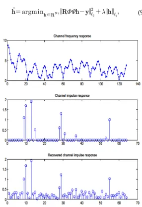
Fig. 1. Channel frequency response and channel impulse response
in (6).
Ⅳ. Performance Enhancement Scheme
In this section, we suggest two approaches to enhance the UWB channel measurements and modeling from UWB-CS system as we presented in previous section. One is the scheme to increase the time resolution using CZT and the other is robust signal recovery scheme.
4.1 CZT for ToA estimation of CIR
From (8), the channel impulse response is estimated through the solution with the Fourier basis for the expansion basis and the canonical basis for sampling basis . In the frequency domain, the time domain resolution is constrained by bandwidth and number of sampling.
When the time-domain response over part of the time period is desired, the chirp-z transform (CZT) is preferred, providing flexibility in the choice of time-domain parameters with the cost of longer computational time as compared with inverse fast Fourier transform (IFFT)[10,12,13]. The CZT transform is defined on z-plane contour with variable amplitude and phason on z-plane contour with the initial amplitude ⋅ and depending on the phase sampling density
⋅ , spirals in or out with respect to the origin. Here is initial frequency.
Thus CZT has advantages when the time function is plotted with high resolution over a small part of the periodic time. Unfortunately, the CZT basis cannot replace into the expansion basis directly.
The reason why we can not apply the CZT directly, is well illustrated in Appendix A. Therefore, the proposed system employs the general IFFT as expansion basis in CS algorithm for recovery the frequency response and then apply the CZT on recovered frequency domain signal by simple FFT to increase the resolution in ToA estimation.
4.2 Robust Signal Recovery from Measured Signal
In general, the measured data is completely
recovered from the partial data through
minimization under the assumption; the original signal is sufficiently sparse and the pair of the expansion basis and the sampling basis has maximal incoherence. Sometimes, one can simply calculate by taking the inverse DFT (IDFT) of .
The optimum - sparse approximation of using this basis can be trivially determined by keeping the
largest values of the IDFT of [13] as shown the Fig. 1. The middle figure is real sparse time domain CIR and top figure is the frequency response of that.
Although, the largest values of original signal can be extracted using only simple IDFT, there are redundant values which can not neglect as shown in bottom figure. Moreover, this paper wish to estimate the ToA values where the non-negligible terms lead dominant error in. Therefore, we consider the robust recovery by remove small power signals seemed to be noise signal.
When the noise exists, the optimization problem of the recovery equation (8) is solved by dual Lagrange multiplier:
∈
(9)
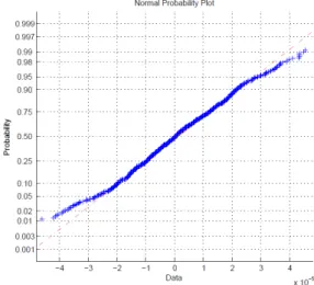
Fig. 2. Normal probability of residual signal of where is coefficient of Lagrange multiplier. The
solution is a function of the parameter . Thus, choosing the appropriate parameter of is important for the solve the optimization problem, but the parameter that makes this problem equivalent cannot be known a priori. However, when sensing matrix,
, is orthogonal and the distribution of noise level is Gaussian, the choice can be determined as a certain value[17]. Donoho proposed a method for reconstructing an unknown functions from noisy data using soft thresholding method[17]. Let set the noisy signal model as follows :
⋅ (10)
where is a with Gaussian noise with zero mean and unit variance and is the noise level. Here, we wish to find an estimate with small mean-squared error as follows:
∥ ∥
(11)
From the (9), the squared error term is controlled by . Specifically, under the assumption that the noise has white Gaussian distribution, the probability of error satisfies that[18]
∥∞∥≤→ (12)
where infinite norm of subscript of is the generalization of the norm to an infinite number of components leads to the spaces.
Therefore, motivated by the (12), the noise level of (10) is replaced by ⋅. Let apply the definition of the soft threshold nonlinearity[18] as
┴ ∥∥ (13)
Here sgn is the sign function that extracts the sign of a real number and subscript + means forward positive sequence so that the noisy coefficients towards 0 by an amount threshold is
.
It means that the noisy coefficients towards 0 by an amount threshold is . Under the two need conditions; one is that the sensing matrix is orthogonal for ∥ ∥
∥ ∥
where
and the other is that the noise has Gaussian distributions, the threshold in (13) can be defined as ⋅ with arbitrary coefficient of . To confirm the assumption, we experiment the noise distribution using 'normplot' commend which is the graphical method used in MATLAB for comparing two probability distributions.
Fig. 2 shows the norm plot of the residual in (11) and it can be verify that the has Gaussian distribution. From that numerical analysis, it is evident that the soft threshold method can be applied in our proposed system. In addition, suppose that the orthogonal sensing matrix has full rank, the noise level is within the power of small number of measured signals, ∈∥∥Finally, the threshold for enhance the performance of CS, is defined as follows:
⋅∥∥⋅ ≤ ≤
(14)
where is the arbitrary coefficient which can adjust the noise threshold is proportiaonl to derived soft
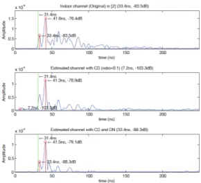
Fig. 3. Channel Impulses response with 500 MHz
Fig. 4. Channel Impulses response with 5GHz threshold and it is obtained through the empirical
results.
Ⅴ. Performance Comparison Applying Soft Threshold Method
The proposed scheme which recovers the frequency channel response using CS algorithm is compared with general CS and the enhanced CS with soft threshold. For the -norm minimization methods, we apply the SPGL1 Matlab solver that can be readily employed[14]. For the measurement in frequency domain, we use Rohde & Schwarz ZVB20 VNA in where the time required to sweep 3-8 GHz band is 5.176 s with a 1 MHz frequency sampling interval and 1 kHz measurement bandwidth.
5.1 Estimated CIR in different BW
Fig. 3 and Fig. 4 show the CIR for three different measurement system with two different bandwidth (BW), namely, 500 MHz and 5 GHz. For the case of CS with denoising scheme (DN) which applying soft thresholding method, the ability to recover the channel response is enhanced comparing with simple CS algorithm case, because the denoising scheme removers the residual terms which can induce enormous errors in delay estimation. In addition, a general fact that has been noticed in this analysis
subsection is that, as the bandwidth of the measurement system increase, the error timing estimation decreases due to enhanced time-domain resolution. For example, at 500 MHz, the detected first arrival time is 33.4 ns in original case and denoising scheme, whereas the case of 5 GHz finds closer delay, 31.7 ns and 32 ns at original case and denoising case.
5.2 Mean and STD of distance error in different BW
Through the Fig. 5-8, the mean and standard deviation (STD) of distance error according to different CS ratio and different BW. Fig. 5 shows the ability to estimate ToA with very small ratio, 0.1 and 0.2. In fact, when the ratio is 0.1, the CS scheme and denoising scheme has mean error of ten times and six times of that of original modeling. In this case, even the increase of BW do not lead the performance enhancement. If the ratio is 0.2, location error of denoising decrease more fast than that of CS scheme. However, both cases still have serious problem for ToA estimation. Fig. 6 shows the mean and std of distance error with over 0.4 ratio. For this case, the estimation performance of middle ratio outperforms the small ratio case significantly.
Especially, the denoising scheme with over 0.4 ratio approaches to the performance original case
Fig. 5. Mean and STD of Distance error with ratio = 0.1, 0.2
Fig. 6. Mean and STD of Distance error with ratio = 0.4, 0.6
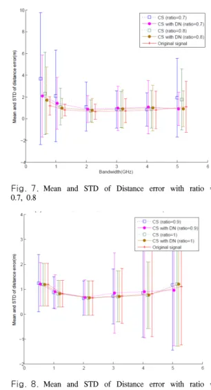
Fig. 7. Mean and STD of Distance error with ratio = 0.7, 0.8
Fig. 8. Mean and STD of Distance error with ratio = 0.9, 1
after 2 GHz. It is evident that the modified scheme can recover the frequency channel response perfectly using only less than half of measured signal.
Interestingly, the error of simple CS system also drops to values below 3 m significantly. In addition, the overall std of distance error is reduced as increase the BW, and the std values of denoising scheme is smaller than that of simple CS recover scheme, even both scheme have same mean error values.
Naturally, the higher ratio cases show much better performance as shown in Fig. 7 and Fig. 8. By examining Fig. 7, it is clear that the mean error of three cases almost same whereas the std values of error are different. This phenomenon means the CS
case has several severe error. Finally, with highest ratio, the mean and std of error almost same values over all possible BW as shown in Fig. 8.
5.3 Distance error in different measurement range power of first arrived signal
To further analyze, Fig. 9~12 depict the distance error for different distance of transmitter antenna and receiver antenna or power of first arrived signal.
Based on the observation of above experiment, we consider 0.4 ratio case where the distance error start to reduce fast.
Fig. 9 and Fig. 10 show distance error with regard to measurement range, which means distance of first arrived signal. The denoising scheme performs significantly better than the CS scheme and
Fig. 9. Distance error vs distance between tx and rx when ratio = 0.4 and BW =[0.5 1 2]GHz
Fig. 10. Distance error vs distance between tx and rx when ratio = 0.4 and BW =[3 4 5]GHz
Fig. 11. Mean and standard derivation of ToA estimation error when ratio = 0.4 and BW =[0.5 1 2]GHz
Fig. 12. Mean and standard derivation of ToA estimation error when ratio = 0.4 and BW = [3 4 5]GHz
the overall error decrease as increase the BW. In 5GHz BW, the errors occur in only 8 points among total 80 measurement trials even with small error values as shown the bottom figure of Fig. 9. In the other hand, when the BW is 0.5, 1, 2 GHz, the CS system has large value of error which are increase following the distance between transmitter and reviver.
Fig. 10 shows the distance error with BW = [3,4,5] GHz. In this category, both distance error of two system become smaller than that of narrow BW case. The error of CS case increase as further distance due to the small received power, but, in the
denoising case, that trend can not observed much small errors. Importantly, the overall distance error do not thoroughly depend on the distance between transmitter and receiver, because UWB channel measurement experimental is performed in indoor environment which severely undergo the dense multi-path fading.
Alternatively, Fig. 11 and Fig. 12 show distance error according to different power of first arrival signal with also 0.4 ratio. The vertical line is the threshold value for ToA estimation. Note again, the
Fig. 13. Cumulative Distance Function of ToA estimation error when ratio = 0.4 and BW =[0.5 1 2]GHz
Fig. 14. Cumulative Distance Function of ToA estimation error when ratio = 0.4 and BW =[3 4 5]GHz
error decrease as increase the BW and receiver power and denoising case has better performance than that of CS case. It is obvious that the estimated error of ToA occurs near the noise threshold level.
Differing from Fig. 11 and Fig. 12, the ToA estimation performance depends on received power linearly more than distance. By examining the two figure, over the -100dB received power, there are few errors. For example, at 5 or 6GHz, any distance error do not occur, that is, the estimation performance is perfect with only 40% samples, although it appears, the value is very small.
5.4 Cumulative Distribution Function
Finally, we analyze the CDF of distance error to observe the optimal CS ratio or possible error bound at the same time. Fig. 13 and Fig. 14 show the CDF of distance error for different BW and CS ratio. A general fact that has been noticed in the analysis section is that, as the CS ratio and BW increase, the corresponding estimation error decreases. For a denoising case, if the ratio is above 0.4, 80 % of distance error drops to below 5 m and drops significantly for overall BW. The CS case has large error even BW is large, whereas the denoising case has almost within 3m error from above 0.4 ratio for whole BW. Especially, at 6, 7, 8GHz, that is BW is 3,4,5 GHz, the case with over 0.4 ratio has almost
same performance as original signal. In addition, the ratio factor of proposed system is more dominant factor than BW criterion. Note that the proposed simple CS scheme reveal a meaningful performance from 0.6 ratio and the enhanced scheme find the exact ToA from 0.4 ratio.
Ⅵ. Conclusion
Ultra-wideband (UWB) technology has been considered as a promising candidate technology for short-range indoor wireless communications. Due to the characteristic of extremely broad bandwidth, the considerate system have to reduce the processing burden because of high sampling rate for practical implementation. In this paper, we proposed the efficient low complexity channel modeling method.
For the channel modeling using frequency measurement signal, the basic frequency measurement system based on compressive sensing algorithm was studied by using the sparsity of time-domain response of UWB. The basic system was established by two steps: recovery of frequency measurement and CIR modeling using CZT. In addition, to enhance the ability to recover of CS, the denoising CS scheme was proposed applying the soft-thresholding method and the threshold to minimize the estimation residual was defined
mathematically. Using the proposed CS based channel modeling method, the indoor UWB channel was measured in real experiment and the quantitative analysis was shown under various conditions.
Appendix-A : The analysis of Chirp-z transform Since the CZT is the general form of z-transform, the discrete z-transform equation can be expressed as
∞ ∞
(15)where the general form of
⋯ and the arbitrary complex numbers and . When , the result corresponds to the discrete Fourier transform(DFT) as follows:
∞ ∞
⋯ (16)where is the -th roots of unity.
If we interest the time domain signal for periodic time , the periodic time is equal to
and ⋅ . From that result, it is known that time domain resolution constrained by the frequency domain resolution, . Thus the equation of discrete signal response in frequency domain is represented as follows:
(17)
For the simple equation, let us use the Bluestein substitution for the exponent of ,
(18)
The (17) can then be rewritten,
(19)
After redefining as
the (19) is represented by convolution with and like as:
⋅⊗ (20)
Therefore, the initial amplitude become
⋅ and the phase sampling density . The general z-plane contour begins with the point and depending on the value of , spirals in or out with respect to the origin. CZT has advantages when the time function is plotted with high resolution over a small part of the periodic time.
If we change the representation basis into CZT matrix , the desired time domain signal can be obtained directly using the inverse CZT matrix.
Unfortunately, however, that the performance degrades because the CZT matrix contains components between only two arbitrary frequencies as :
(21)
Let set the CZT matrix as and the inverse CZT matrix as . The matrix composed with and inverse matrix of that has relationship
⋅≠ , where is unitary matrix, because it contains partial information which lead the error in recovery process in CS. Therefore, the proposed system do not apply the inverse CZT matrix as expansion basis and employ the general IFT basis in CS algorithm to estimate the time impulse response from frequency measurements. And then
the frequency response is recovered using simple FFT basis and then the CZT is applied to increase the resolution in ToA estimation based on recovered frequency response.
References
[1] R. J. Barton, Design and analysis of an ultra-wideband location and tracking system for space-Based applications, NASA Johnson Space Center, Houston, TX August 31, 2005.
[2] N. Alsindi, X. Li, and K. Pahlavan, “Analysis of time of arrival estimation using wideband measurement of indoor radio propagations,”
IEEE Trans. Instrumentation and Measurement, vol. 56, no. 5, pp. 1537-1545, 2007.
[3] B. Alavi K. Pahlavan, “Modeling of the distance error for indoor geolocation,” IEEE Wirel. Commun. Netw. (WCNC), pp. 668-672, Mar. 2003.
[4] K. Pahlavan, X. Li, and J.-P. Makela “Indoor geolocation science and technology,” IEEE Commun. Mag., vol. 40, no. 2, pp. 112-118, 2002.
[5] J. H. Kim, I. S. Back, and S. H. Cho,
“Compensation of received signal attenuation by distance using UWB radar” in Proc. KICS, pp. 282-283, Feb. 2012.
[6] M.-K. Kang, J. Kang, S. Lee, Y. Park, and K.
Kim, “A study on kalman filter in IR-UWB RTLS,” in Proc. KICS, pp. 996-997, Jun. 2011.
[7] D.-J. Kang, K.-J. Park, and H.-J. Park, “A study on ways to correct UWB position estimation techniques in indoor environment,”
in Proc. KICS, pp. 167-168, Feb. 2012.
[8] V. Bataller, A. Munoz, N. Ayuso, and J. L.
Villarroel, “Channel estimation in through- the-earth communications with electrodes,”
PIERS Online, vol. 7, no. 5, pp. 486-490, 2001.
[9] E. J. Candes and M. B. Wakin, “An introduction to compressive sampling,” IEEE Signal Processing Mag., pp. 21-30, Mar. 2008.
[10] X. Li and K. Pahlavan, “Super-resolution TOA estimation with diversity for indoor geolocation,” IEEE Trans. Wirel. Commun.,
vol. 3, no. 1, pp. 224-234, Jan. 2004.
[11] K. Pahlavan and A. Levesque, Wireless Information Networks, NY: Wiley, 1995.
[12] B. Ulriksson, “Conversion of frequency-domain data to the time domain,” in Proc. IEEE, vol.
74, pp. 74-76, Jan. 1986
[13] C. R. Berger and Z. Wang and Jianzhong Huang, and S. Zhou, “Application of compressive sensing to sparse channel estimation,” in Proc. IEEE Commun. Mag., pp. 164-174, Nov. 2010.
[14] M. P. Friedlander and E. van den Berg, SPGL1: A solver for large-scale sparse reconstruction, available at http://www.cs.ub c.ca/labs/scl/spgl1.
[15] S. J. Howard and K. Pahlavan, “Measurement and analysis of the indoor radio channel in the frequency Domain,” IEEE Trans. Instru- mentation and Measurement, vol. 39, no. 5, Oct. 1990.
[16] A. A. M. Saleh and R. A. Valenzuela, “A statistical model for indoor multipath propagation,” IEEE J. Select. Areas Commun., vol. 5, no. 2, pp. 128-137, Feb. 1987.
[17] D. L. Donoho, “De-noising by soft thresholding,” in Proc. IEEE Trans. Inform.
Theory, vol. 41, no. 3, pp. 613-627, May 1995.
[18] S. S. Chen, D. L. Donoho, and M. A.
Saunders, “Atomic Decomposition by Basis Pursuit,” SIAM J. Sci. Comput., vol. 20, no. 1, pp. 33-61, Jul. 2006.
김 수 진 (Sujin Kim)
2006년 2월:이화여자 대학교 정보통신 공학과 학사 2008년 2월:한국과학기술원 정
보통신학과 석사
2012년 8월:한국과학기술원 정 보통신학과 박사
현재:국방과학연구소 선임연 구원
<관심분야> 근거리 무선통신 시스템, 실내위치 추정
명 정 호 (Jungho Myung)
2007년 2월:충남대학교 전자 과 학사
2009년 2월:한국과학기술원 정 보통신학과 석사
2013년 8월:한국과학기술원 전 자과 박사
현재:전자통신연구원 연구원
<관심분야> Relay Transmission, Cognitive Radio (CR)
강 준 혁 (Joonhyuk Kang)
1991년 2월:서울대학교 제어 계측공학 학사
1993년 2월:서울대학교 제어 계측공학 석사
2002년:Texas Austin 전자통 신 정보 시스템공학 박사 현재:한국과학기술원 전자과
교수
<관심분야> CR, MIMO-OFDM, 실내외 측위
성 태 경 (Tae-Kyung Sung)
1984년 2월:서울대학교 제어 계측공학과 학사
1986년 2월:서울대학교 제어 계측공학과 석사
1992년 2월:서울대학교 제어 계측공학과 박사
1997~현재:충남대학교 정보통 신공학과 교수
<관심분야> GPS/GNSS, 지상파 측위, 위치인지 신 호처리
이 광 억 (Kwang-Eog Lee)
1988년 2월:경북대학교 전자 공학과 학사
1990년 2월:경북대학교 전자 공학과 석사 졸업
현재:국방과학연구소 책임연 구원
<관심분야> CR, Dynamic spectrum access
![Fig. 9. Distance error vs distance between tx and rx when ratio = 0.4 and BW =[0.5 1 2]GHz](https://thumb-ap.123doks.com/thumbv2/123dokinfo/5279397.371814/9.799.83.372.89.361/fig-distance-error-vs-distance-ratio-bw-ghz.webp)
![Fig. 13. Cumulative Distance Function of ToA estimation error when ratio = 0.4 and BW =[0.5 1 2]GHz](https://thumb-ap.123doks.com/thumbv2/123dokinfo/5279397.371814/10.799.418.708.99.386/fig-cumulative-distance-function-toa-estimation-error-ratio.webp)
