Article
http://dx.doi.org/10.4217/OPR.2017.39.1.013 Ocean and Polar Research March 2017
Optimal Monitoring Frequency Estimation Using Confidence Intervals for the Temporal Model of a Zooplankton Species Number Based on Operational Taxonomic Units at the Tongyoung Marine Science Station
Hong-Yeon Cho1,2*, Sung Kim3,4, Youn-Ho Lee3,4, Gila Jung3, Choong-Gon Kim3, Dageum Jeong3, Yucheol Lee5, Mee-Hye Kang3, Hana Kim6, Hae-Young Choi3,4, Jina Oh3,
Jung-Goo Myong3,4, and Hee-Jung Choi3
1Ocean Data Science Section, Large Facility Operations and Support Department, KIOST Ansan 15627, Korea
2Integrated Ocean Sciences, University of Science and Technology Ansan 15627, Korea
3Marine Ecosystem and Biological Research Center, Marine Life and Ecosystem Division, KIOST Ansan 15627, Korea
4Marine Biology Sciences, University of Science and Technology Ansan 15627, Korea
5Biological Sciences, College of Natural Sciences, Inha University Incheon 22212, Korea
6Department of Taxonomy and Systematics, National Marine Biodiversity Institute of Korea Seochun 33662, Korea
Abstract : Temporal changes in the number of zooplankton species are important information for under- standing basic characteristics and species diversity in marine ecosystems. The aim of the present study was to estimate the optimal monitoring frequency (OMF) to guarantee and predict the minimum number of spe- cies occurrences for studies concerning marine ecosystems. The OMF is estimated using the temporal number of zooplankton species through bi-weekly monitoring of zooplankton species data according to operational taxonomic units in the Tongyoung coastal sea. The optimal model comprises two terms, a con- stant (optimal mean) and a cosine function with a one-year period. The confidence interval (CI) range of the model with monitoring frequency was estimated using a bootstrap method. The CI range was used as a reference to estimate the optimal monitoring frequency. In general, the minimum monitoring frequency (numbers per year) directly depends on the target (acceptable) estimation error. When the acceptable error (range of the CI) increases, the monitoring frequency decreases because the large acceptable error signals a rough estimation. If the acceptable error (unit: number value) of the number of the zooplankton species is set to 3, the minimum monitoring frequency (times per year) is 24. The residual distribution of the model followed a normal distribution. This model can be applied for the estimation of the minimal monitoring frequency that satisfies the target error bounds, as this model provides an estimation of the error of the zoo- plankton species numbers with monitoring frequencies.
Key words : zooplankton, temporal number of species model, confidence interval, Bootstrap method, optimal monitoring frequency
*Corresponding author. E-mail : [email protected]
1. Introduction
Zooplankton is important as an energy messenger in the food chain of the ocean ecosystem. These zooplanktons live in diverse areas, such as the coastal seas, ranging from the surface to deep bottom layers of the ocean (Nishida and Nishikawa 2011). Despite differences in the diverse environments, the homeostasis in species diversity of zooplankton provides important information for the characteristic analysis of the marine ecosystem, the evolution of the marine organisms and the conservation of the ecosystem (Irigoien et al. 2004; Tittensor et al. 2010).
The zooplankton species diversity considerably varies with changes in the coastal environment and species- specific life cycles (Nogueira 2001; Lo et al. 2004;
Hwang et al. 2011; Lee et al. 2006). The range and frequency are different for the analysis of spatio-temporal changes in species composition. The typical sampling periods range from 4 times (seasonal survey) to 50 times per year within surveyed areas (Moon et al. 2010; Lee et al. 2006; Lee et al. 2012; Hwang et al. 2011).
The ecosystem survey requires an optimal or appropriate monitoring plan for the biological and physiological change analysis because there is a limitation on available cost and labor (Millard and Lettenmaier 1986; Dixon and Chiswell 1996). The increased monitoring numbers for zooplankton reduces the confidence intervals in the estimation error of zooplankton species models based on
the monitoring data. The increase in survey numbers, however, means an increase in time and labor necessary for species identification. Thus, studies on the estimation of the minimum optimal monitoring frequency (OMF) are necessary to target acceptable error boundaries. The aim of the present study was to estimate the OMF to guarantee and predict the minimum number of species needed for studies concerning marine ecosystems. The OMF is estimated using the temporal number of zooplankton species models using the bi-weekly monitored zooplankton species data according to operational taxonomic units in the Tongyoung coastal sea. The confidence interval (CI) of the model with monitoring frequency is estimated using a bootstrap method. The CI is used as the reference to estimate the optimal monitoring frequency.
2. Materials and Methods
Materials
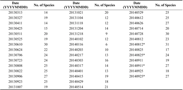
A total of 43 samples were collected nearly bi-weekly using a conical net (front half – cylindrical, connected rear half – conical; mouth diameter, 60 cm; mesh size, 200 µm;
length, 300 cm; vertical towing) attached flowmeter from March, 2013 to September, 2014 in the Tongyoung Marine Science Station of the Korea Institute of Ocean Science and Technology (34o45.80'N, 128o21.45'E) off the Tongyoung coast. The difference in species number may occur depending on the inflow-quantity. However, in the
Table 1. Data set on the number of zooplankton species and sampling dates Date
(YYYYMMDD) No. of Species Date
(YYYYMMDD) No. of Species Date
(YYYYMMDD) No. of Species
20130313 14 20131021 20 20140529 25
20130327 19 20131104 12 20140612 25
20130411 14 20131118 12 20140626 27
20130425 15 20131204 14 20140714 20
20130511 20 20131218 9 20140728 30
20130525 19 20140102 12 20140812 23
20130610 30 20140116 6 20140812* 31
20130624 22 20140203 10 20140825 17
20130706 24 20140217 13 20140825* 24
20130723 24 20140303 16 20140911 19
20130808 25 20140317 14 20140911* 27
20130822 25 20140401 13 20140925 18
20130906 27 20140415 19 20140925* 27
20130923 25 20140429 18
20131007 19 20140514 21
Ref. * = Sampled at different time, but regarded as the same day monitoring data set
present study, the difference was found to be insignificant because the species number of zooplankton reached the saturation level of the rare-faction curve.
The independent zooplankton species were identified by using DNA meta-bar-coding process to be explained in detail below and the number of zooplankton species was obtained after counting the available species numbers obtained (selected data based on the threshold reading numbers) at different sampling times (Table 1; KIOST 2016). The genomic DNA (gDNA) of zooplankton was extracted using the QIAGEN® DNeasy Blood & Tissue KIT (Qiagen, Inc., Valencia, CA). The gDNA was subsequently amplified using a previously described primer set (mlCOIintF and jgHCO2198, Leray et al.
2013). After generating a library using refined PCR products, we sequenced the PCR products according to the protocol of MiSeq (Illumina Inc., San Diego, CA).
The nucleotide sequences for low-quality reads and chimeras were removed using the CD-HIT-OTU program.
Subsequently, clustering was performed based on the Molecular Operational Taxonomic Units (MOTUs) at the 98% similarity level (Li et al. 2012; Blaxter et al. 2005;
Machida et al. 2009). After searching/comparing the NCBI non-redundant database and MegaBLAST MOTUs with these produced MOTUs, the zooplankton species were confirmed (Zhang et al. 2000), and the MOTUs had a pair-wise identity over 97% and query coverage over 90% (Carew et al. 2013).
Methods
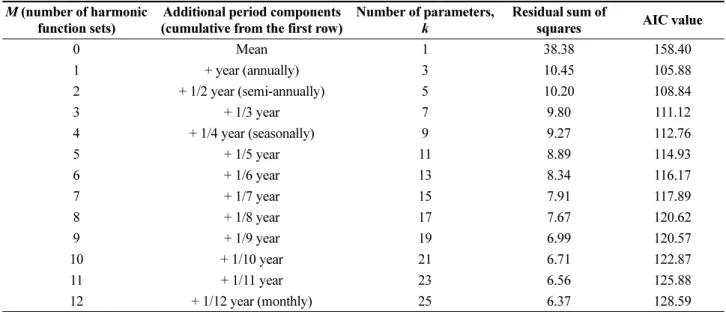
Temporal number of zooplankton species model The simplest model of the number of zooplankton species model is the mean-constant model. This model is has only one parameter, but is optimal because it cannot explain temporal changes, such as seasonal and inter- annual changes. The optimal model was selected based on the AIC (akaike information criteria) values computed using Eq. (1). When the AIC value is minimal, the model can be regarded as optimal (Akaike 1974; Johnson and Omland 2004),
(1) in which, k is the number of the model parameters, n is the size of the data sample (in this study, n = 43), and RSS is the residual sum of squares.
The candidate models comprise the summations of functions with many period components, from the 1-year period to semi-annual, seasonal, and monthly cycle terms.
The optimal model is selected after comparing the AIC
values computed from the possible models. The temporal number of the zooplankton species model can be expressed as Eq. (2), in general form. The parameters are optimally estimated using the least squares method, minimizing the cost function as the residual (error) sum of squares in the given number of the harmonic functions, M, as shown in Eq. (1):
(2)
in which is the number of zooplankton species at time ti ( ), n is the number of samples, is the optimal mean of the number of zooplankton species, M is the number of harmonic functions, and ωj
is the frequency components of the model, defined as 2πj/365.25 (1/days). Aj, φj are the amplitude and phase of the harmonic function with the frequency ωj, respectively; εi is the residual error, defined as the difference between the observed and model- estimated number of zooplankton species at time ti.
The data used in this study were collected for approximately one and a half years. The monitoring date of the data was converted to Julian days to generate intra- annual data. Thus, the model can be considered as a temporal model for understanding intra-annual, not inter- annual, changes. The model can be set up using the number of zooplankton species data accumulated/collected during many years, assuming no trend. Using this model, it is possible to estimate the expected number (reference number) of times and/or samples to satisfy the target error bounds. The normality on the residuals is assessed using KS and Anderson-darling tests with 95% confidence levels in the ‘nortest’ package in R (Juergen and Uwe 2015). This value can be used to estimate the confidence intervals of the model when the error distribution follows a normal distribution.
There are parametric and non-parametric methods for when the temporal number of a species model is assumed to be a harmonic function and not assumed to be another specific function, respectively. The latter is more flexible than the former because the model is not subject to a specific function. However, the non-parametric methods have more complex expression functions, such as the summation form of functions, making statistical inferences difficult because of the lack of supported closed-form of functions (Wand and Jones 1995; Martinez and Martinez 2005). In the present study, the model is estimated using a non-parametric method. These data are subsequently used as the reference model to determine whether estimating AIC=2k n log RSS/n+ ⋅ ( )
NZ( ) Nti Z Ajcos(ωj⋅ti–φj)
j 1=
∑M εi
+ +
= NZ( )ti
i 1 2 … n= , , , NZ
j 1 2 … M= , , ,
( )
the other model using a parametric method is suitable.
This non-parametric model, expressed as a locally smoothed regression curve, can be estimated using the ‘locpoly’
function in R ‘KernSmooth’ package, and ‘smooth’
function (option=‘loess’) supported through MATLAB. In the present study, we estimated the model using the
‘smooth’ function in MATLAB. To generate the smooth curves in data boundaries (times are indicated near the left (1) and right (365) boundaries), the virtual data sets were added to the original data after adjusting the time index.
When the original data set comprises the sampling time in Julian days and number of zooplankton species, the virtual data sets are the same, except for the time. In virtual data, the time was changed to time+365 and time- 365 days, and the data size increased 3-fold.
Confidence interval estimation using the bootstrap method The confidence intervals (CIs, error bounds, also considered as the CI range = the range of the upper and lower limits of the CI) of the temporal number of the zooplankton species (TNZS) model were estimated using the bootstrap method, a powerful method using random re-sampling simulations with substitution when analytical computational methods are not available and the assumption on error distribution is not required. This method is a Monte-Carlo simulation method, estimating the CIs at a given significance level α after computing the specific percentile values of many (about above 1,000 to 1,000,000) simulated results (Efron 1979; Rubinstein and Kroese 2008). This method has been widely used to examine the statistical methods and estimate the optimal monitoring
intervals and CIs with given monitoring intervals for the variation pattern analysis of the environmental and ecological parameters (Anttilla et al. 2012; Dowd et al.
2004; U.S. Environmental Protection Agency 2010; Cho et al. 2013).
In the present study, the 90%-confidence intervals (significance level 10%, double-sided) of the mean error bound of the model were estimated. The mean error bound is defined as the error bound using the optimal parameter estimation for this model. The simulation number used was 100 for the sake of computational efficiency. The larger the number is, the lower the computational efficiency becomes. The simulation number determines the mean error bound of the estimated error bounds and is suggested analytically as with the assumption of the normality of the error bound distribution. In this method, however, the 95%-CI of the mean error bound was also estimated using the bootstrap method for consistency. In this case, the simulation number was also 100. The CI obtained using the bootstrap method is the error range associated with the model selection (optimal estimation), and this value is different from the error obtained upon estimation of the number of zooplankton species using the model.
3. Results
Estimation error resulting from the level (order) of model complexity
The estimated number of zooplankton species using candidate models was compared with the observed
±1.96σˆ/ n
Table 2. Changes in the AIC values with the number of harmonic functions, M M (number of harmonic
function sets)
Additional period components (cumulative from the first row)
Number of parameters, k
Residual sum of
squares AIC value
0 Mean 1 38.38 158.40
1 + year (annually) 3 10.45 105.88
2 + 1/2 year (semi-annually) 5 10.20 108.84
3 + 1/3 year 7 9.80 111.12
4 + 1/4 year (seasonally) 9 9.27 112.76
5 + 1/5 year 11 8.89 114.93
6 + 1/6 year 13 8.34 116.17
7 + 1/7 year 15 7.91 117.89
8 + 1/8 year 17 7.67 120.62
9 + 1/9 year 19 6.99 120.57
10 + 1/10 year 21 6.71 122.87
11 + 1/11 year 23 6.56 125.88
12 + 1/12 year (monthly) 25 6.37 128.59
numbers after optimal parameter estimation. The estimation error (residual) sum of squares and AIC values are shown in Table 2. The optimal model was selected as a function only with including the 1-year period component because the AIC value was minimal at that condition. The function is shown in Eq. (3), and the simplest mean model is also expressed in Eq. (4) for a basic comparison.
(3)
(4) Based on the optimal model, the timings (dates) of the maximum and minimum number of zooplankton species were calculated using the conditions
= 0 and , respectively. The
computed dates in Julian days were 202 (21st July) and 19 (19th January), respectively, and the numbers of species observed on those dates were 26 (maximum) and 10 (minimum), respectively.
The mean model showed a large AIC value, reflecting large residuals (variance of the data) defined as differences in the observed and estimated number of the zooplankton species. Although the residuals of the more complex models with more parameters decreased, the quantitative effects were not large compared with the increase in the number of parameters used to calculate the AIC values.
However, the model estimated using the non-parametric method showed different shapes for the slope of the increasing and decreasing stages and the peak pattern (more flat than the parametric model). However, the non- parametric model was within the 95% error bounds of the NZ( ) 17.95 7.86 costi 2πti
365.25 --- 2.81+
⎝ ⎠
⎛ ⎞
⋅ N 0 3.19( , 2)
+ +
=
NZ( ) 17.95 7.86 costi 2π 365.25
--- t(i–201.65)
⎝ ⎠
⎛ ⎞
⋅ N 0 3.19( , 2)
+ +
=
NZ( ) 19.63 N 0 6.20ti = + ( , 2)
2πti/365.25
( ) 2.81+
2πti/365.25
( ) 2.81+ =π
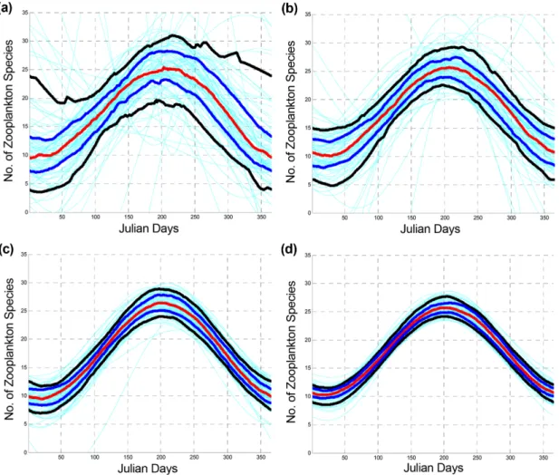
Fig. 1. CI curves (90%) of the error bounds of the model with the number of survey times. The red line represents the optimal model function. The black and blue lines show the upper and lower limits of the model at 10%
and 25% significance levels, respectively. The cyan lines represent the estimated models using the generated samples and the bootstrap method. (a) Seasonal survey (n = 4), (b) Bi-monthly survey (n = 6), (c) Monthly survey (n = 12), and (d) Bi-weekly survey (n = 24)
parametric model. The residual components of the optimal model followed the normal distribution based on the KS- test and Anderson-Darling test in terms of 95% confidence intervals (5% significance level). The CIs (estimation error bounds) were approximately ±2 number of species.
Confidence interval estimation of the model based on survey times
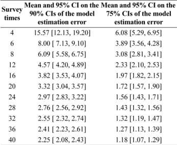
The survey times are the sample numbers used to determine the confidence intervals. We assumed that the total data on the number of zooplankton species collected at Tongyoung Marine Science Station constituted the reference population. The 90% CI estimation of the model was determined using a bootstrap method. The CI decreased with increasing survey times from 4, 6, and 12 to 24 times (Fig. 1). The analysis of the variation pattern was performed using both 75 and 90% confidence intervals. Both CIs decreased, showing power function patterns. For fewer survey times, the CI rapidly increased.
Subsequently, for survey times longer than 24 times, the CI slowly decreased to a negligible extent. The CI with survey times provided in Table 3 can be fitted with the power function shown in Eq. (5). The exponents of the functions were -0.76 and -0.67 at the 90% and 75%
confidence intervals, respectively.
(5)
in which, Y denotes the CIs, the subscripts of Y (90 and 75) are the percentage values of the confidence levels, X is the number of surveys (survey times), and R2 is the coefficient of determination. If the acceptable error (unit:
number value) of the number of the zooplankton species is set to 3, the minimum monitoring frequency (times per year) is 24.
4. Discussions
Basic information on the number of zooplankton species is essential for understanding the characteristic marine ecosystems. For diverse analyses, such as that of the life cycle, influence on the species due to seasonal environmental parameters (e.g., water temperature) and habitat changes are likely derived using these data (Allan 1976; Conover and Huntley 1991; Machida et al. 2009).
In addition, information on the characteristic parameters of zooplankton can be used as indicators for the assessment and management of the environmental and ecological impacts of global warming and ocean acidification (particularly, decreasing pH, not yet reaching a neutral pH of 7.0) (Link et al. 2002; Bucklin et al. 2010).
However, the accurate identification of zooplankton species diversity is difficult because the number of species increases following the rarefaction curve. The number of species is not linearly proportional to the survey times and the amount (weight) of the samples (Machida et al. 2009).
In the present study, we estimated the optimal survey frequency necessary for the analysis of the species composition and number of species using data for the number of zooplankton species monitored bi-weekly in the Marine Research Platform in the Tongyoung coastal sea. The size of the data set was 43. The optimal model for the temporal number of zooplankton species was selected based on these data. The CI due to survey times was estimated using a bootstrap method (Efron 1979).
Based on the optimal model, the dates for the maximum and minimum number of zooplankton species can be calculated. The computed dates, as Julian days, were 202 (21st July) and 19 (19th January), respectively, and the numbers of species observed on those dates were 26 and 10, respectively. These results were strongly expected, as these numbers are approximately consistent with typical water temperature variation patterns. The model estimated using a non-parametric method showed different shapes in the slope of the increasing and decreasing stages and the peak patterns (more flat than the parametric model), as shown in Fig. 2. However, these differences were not Y90=34.01⋅X–0.76 (R2=0.960)
Y75=13.41⋅X–0.67 (R2=0.985)
Table 3. Mean, lower and upper limits of the model esti- mation error with the number of survey times Survey
times
Mean and 95% CI on the 90% CIs of the model
estimation error
Mean and 95% CI on the 75% CIs of the model
estimation error 4 15.57 [12.13, 19.20] 6.08 [5.29, 6.95]
6 8.00 [ 7.13, 9.10] 3.89 [3.56, 4.28]
8 6.09 [ 5.58, 6.75] 3.08 [2.81, 3.41]
12 4.57 [ 4.20, 4.89] 2.33 [2.10, 2.53]
16 3.82 [ 3.53, 4.07] 1.97 [1.82, 2.15]
20 3.32 [ 3.04, 3.57] 1.72 [1.57, 1.90]
24 2.97 [ 2.83, 3.22] 1.56 [1.43, 1.71]
28 2.76 [ 2.56, 2.92] 1.43 [1.32, 1.56]
32 2.55 [ 2.32, 2.74] 1.32 [1.19, 1.47]
36 2.41 [ 2.23, 2.61] 1.27 [1.13, 1.39]
40 2.25 [ 2.08, 2.43] 1.18 [1.07, 1.29]
Ref. The value shown in the cell is the mean, and the values shown in the bracket [ ] are the lower and upper limits, respectively. These values correspond to the number of species
statistically significant. The CI of the model decreased with increasing survey time. The residual distribution of the model followed a normal distribution. In general, the minimum monitoring frequency (numbers per year) directly depends on the target (acceptable) estimation error. When the acceptable error (range of the CI) increases, the monitoring frequency decreases. Based on the results of this study, the minimum frequency is 24. The uncertainty of the annual fluctuation numbers increased as the frequency of zooplankton surveys decreased (Fig. 1).
The uncertainty level should be low for the accurate analysis of an ecosystem using the number of species and species composition data for zooplankton.
The species numbers and diversity indices have been suggested as the basic statistics for the analysis of the diverse ecological research fields on zooplankton (Lee et al. 2006; Moon et al. 2010; Lee et al. 2012). However, it is difficult to directly compare these values. The numbers of species are expected to show a large fluctuation with the number of surveys (frequency) based on the model results (see Fig. 1) for the zooplankton occurrence suggested in the present study. Therefore, this model might reflect the determination of the optimal survey times necessary for understanding the ecological zooplankton structure.
5. Conclusions and recommendations
The optimal temporal model for the number of zooplankton species in Tongyoung coastal sea can be
expressed as the following model-function:
The minimum monitoring number is 24 when the acceptable model estimation error is set to 3. It means that at least 24 monitoring times per year (approximately 2 times per month) are required to keep the errors (fluctuation size) below 3. Based on the results of this study, bi-weekly monitoring data are considered sufficient to quantify the annual variation of the number of zooplankton species without any significant error. However, since this study was carried out using only one coastal monitoring station data, it is necessary to be careful to use it as a monitoring standard for the whole coastal waters in Korea. In order to set more general criteria, a comparative study with the results of analysis using data of many different coastal waters is highly required. In addition, an error analysis using data with more short-term time scales (smaller than two weeks interval) is highly recommended.
In practice, a continuous monitoring system is the best, when possible.
Acknowledgements
This research was financially supported in part through the “Development of Korea Operational Oceanographic System (KOOS), Phase 2” project (PM59691), and also funded by the Ministry of Oceans and Fisheries, Korea
NZ( ) 17.95 7.86 costi 2π 365.25
---(ti–201.65)
⎝ ⎠
⎛ ⎞
⋅ +
= Fig. 2. Optimal model for the temporal number of zooplankton species
and a grant from the Korea Institute of Ocean Science and Technology (PE99311).
References
Akaike H (1974) A new look at the statistical model identification. IEEE T Automat Contr AC-19(6):716−723 Allan JD (1976) Life history patterns in zooplankton. Am
Nat 110(971):165−180
Anttila S, Ketola M, Vakkilainen K, Kairesalo T (2012) Assessing temporal representativeness of water quality monitoring data. J Environ Monit 14:589−595
Blaxter M, Mann J, Chapman T, Thomas F, Whitton C, Floyd R, Abebe E (2005) Defining operational taxonomic units using DNA barcode data. Philos Transactions R Soc B: Biol Sci 360(1462):1935−1943
Bucklin A, Nishida S, Schnack-Schiel S, Wiebe PH, Lindsay D, Machida RJ, Copley NJ (2010) A census of zooplankton of the global ocean. In: McIntyre A (ed) Life in the world's oceans: diversity, distribution, and abundance.
Wiley-Blackwell Pub, Chichester, pp 247−265
Carew ME, Pettigrove VJ, Metzeling L, Hoffmann AA (2013) Environmental monitoring using next generation sequencing: rapid identification of macroinvertebrate bioindicator species. Front Zool 10(1):45
Cho H, Jeong WM, Jun KC (2013) Relationship analysis on the monitoring period and parameter estimation error of the coastal wave climate data. J Kor Soc Coast Ocean Eng 25(1):1−6
Conover RJ, Huntley M (1991) Copepods in ice-covered seas-distribution, adaptations to seasonally limited food, metabolism, growth patterns and life cycle strategies in polar seas. J Mar Syst 2:1−41
Dixon W, Chiswell B (1996) Review of aquatic monitoring program design. Water Res 30(9):1935−1948
Dowd M, Martin JL, Legresley MM, Hanke A, Page FH (2004) A statistical method for the robust detection of interannual changes in plankton abundance: analysis of monitoring data from the Bay of Fundy, Canada. J Plankton Res 26(5):509−523
Efron B (1979) Bootstrap methods: another look at the Jackknife. Ann Stat 7(1):1−26
Hwang MO, Shin K, Baek SH, Lee W-J, Kim S, Jang M-C (2011) Annual variations in community structure of mesozooplankton by short-term sampling in Jangmok Harbor of Jinhae Bay. Ocean and Polar Res 33:235−253 Irigoien X, Huisman J, Harris RP (2004) Global biodiversity
patterns of marine phytoplankton and zooplankton.
Nature 429:863−867
Johnson JB, Omland KS (2004) Model selection in ecology and evolution. Trends Ecol Evol 19(2):101−108
Juergen G, Uwe L (2015) Nortest: tests for normality. R package version 1.0.3. http://CRAN.R-project.org/package=
nortest Accessed 3 Sep 2016
KIOST (2016) Development of in-situ diagnostic techniques on the dynamics of marine pelagic ecosystem structure.
Korea Institute of Ocean Science and Technology, BSPE 99311-10858-3, 185 p
Lee CR, Park C, Yang SR, Sin YS (2006) Spatio-temporal variation of mesozooplankton in Asan Bay. The Sea 11:1−10
Lee JK, Park C, Lee DB, Lee SW (2012) Variations in plankton assemblage in a semi-closed Chunsu Bay, Korea.
The Sea, J Kor Soc Oceanogr 17:95−111
Leray M, Yang JY, Meyer CP, Mills SC, Agudelo N, Ranwez V, Boehm JT, Machida RJ (2013) A new versatile primer set targeting a short fragment of the mitochondrial COI region for metabarcoding metazoan diversity: application for characterizing coral reef fish gut contents. Front Zool 10(1):34
Li W, Fu L, Niu B, Wu S, Wooley J (2012) Ultrafast clustering algorithms for metagenomic sequence analysis.
Brief Bioinform 13(6):656−668
Link JS, Brodziak JKT, Edwards SF, Overholtz WJ, Mountain D, Jossi JW, Smith TD, Fogarty M (2002) Marine ecosystem assessment in a fisheries management context. Can J Fish Aquat Sci 59:1429−1440
Lo WT, Chung CL, Shih CT (2004) Seasonal distribution of copepods in Tapong Bay, southwestern Taiwan. Zool Stud 43:464−474
Machida RJ, Hashiguchi Y, Nishida M, Nishida S (2009) Zooplankton diversity analysis through single-gene sequencing of a community sample. BMC Genomics 10(1):438
Martinez WL, Martinez AR (2005) Exploratory data analysis with MATLAB. Chapman Hall/CRC, Boca Raton, 405 p Millard SP, Lettenmaier DP (1986) Optimal design of
biological sampling programs using the analysis of variance. Estuar Coast Shelf Sci 22(5):637−656
Moon SY, Oh H-J, Soh HY (2010) Seasonal variation of zooplankton communities in the southern coastal waters of Korea. Ocean and Polar Res 32:411−426
Nishida S, Nishikawa J (2011) Biodiversity of marine zooplankton in Southeast Asia (Project-3: plankton group).
In: Nishida S, Fortes MD, Miyazaki N (eds) Coastal marine science in Southeast Asia-synthesis report of the Core University Program of the Japan Society for the Promotion of Science, 2001−2010 Coastal Marine Science.
Terrapub, Tokyo, pp 59−71
Nogueira MG (2001) Zooplankton composition, dominance and abundance as indicators of environmental compart- mentalization in Jurumirim Reservoir (Paranapanema River), São Paulo, Brazil. Hydrobiologia 455:1−18 Rubinstein RY, Kroese DP (2008) Simulation and the Monte
Carlo method. Wiley, Hoboken, 372 p
Tittensor DP, Mora C, Jetz W, Lotze HK, Ricard D, Berghe EV, Worm B (2010) Global patterns and predictors of marine biodiversity across taxa. Nature 466:1098−1101 U.S. Environmental Protection Agency (2010). Sampling and
consideration of variability (temporal and spatial) for monitoring of recreational waters, EPA-823-R-10-005.
https://www.epa.gov/sites/production/files/2015-11/docu- ments/sampling-consideration-recreational-waters.pdf Accessed 6 Jun 2016
Wand MP, Jones MC (1995). Kernel smoothing. Chapman
& Hall/CRC, Boca Raton, 224 p
Zhang Z, Schwartz S, Wagner L, Miller W (2000) A greedy algorithm for aligning DNA sequences. J Comput Biol 7(1/2):203−214
Received Dec. 19, 2016 Revised Mar. 5, 2017 Accepted Mar. 16, 2017