Development of Land fog Detection Algorithm based on the Optical and Textural Properties of Fog using COMS Data

1. Introduction

Fog is a meteorological phenomenon in which small water droplets (or super-cooled water droplets or ice crystals) are suspended in the atmosphere with the

lower boundary touching the Earth’s surface with horizontal visibility of less than 1 km (KMA, 2009).

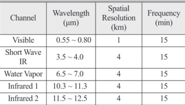
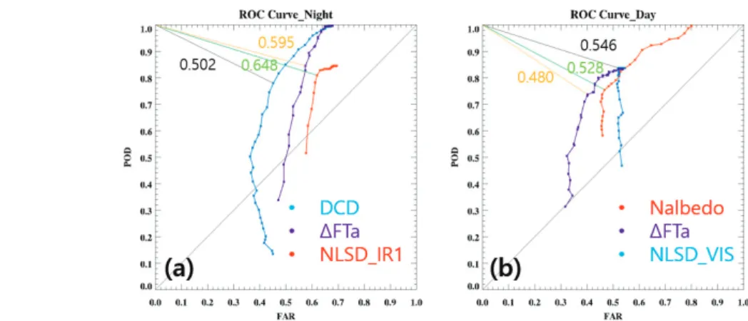
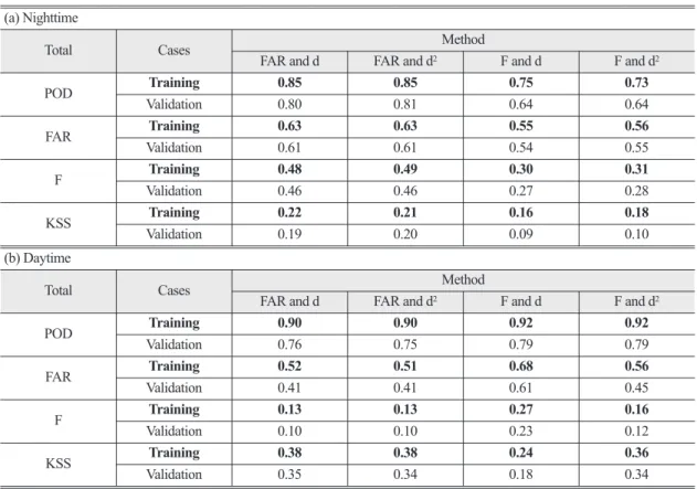
Fog occurring at close proximity to the Earth’s surface impairs visibility and, consequently, critically affects most transportation, such as automobiles, ships, and Abstract : We developed fog detection algorithm (KNU_FDA) based on the optical and textural properties of fog using satellite (COMS) and ground observation data. The optical properties are dual channel difference (DCD: BT3.7 - BT11) and albedo, and the textural properties are normalized local standard deviation of IR1 and visible channels. Temperature difference between air temperature and BT11 is applied to discriminate the fog from other clouds. Fog detection is performed according to the solar zenith angle of pixel because of the different availability of satellite data: day, night and dawn/dusk. Post-processing is also performed to increase the probability of detection (POD), in particular, at the edge of main fog area. The fog probability is calculated by the weighted sum of threshold tests. The initial threshold and weighting values are optimized using sensitivity tests for the varying threshold values using receiver operating characteristic analysis. The validation results with ground visibility data for the validation cases showed that the performance of KNU_FDA show relatively consistent detection skills but it clearly depends on the fog types and time of day. The average POD and FAR (False Alarm Ratio) for the training and validation cases are ranged from 0.76 to 0.90 and from 0.41 to 0.63, respectively. In general, the performance is relatively good for the fog without high cloud and strong fog but that is significantly decreased for the weak fog. In order to improve the detection skills and stability, optimization of threshold and weighting values are needed through the various training cases.

Key Words : Fog, detection, optical and textual properties, visibility meter, COMS

Received July 31, 2017; Revised August 4, 2017; Accepted August 9, 2017.

†

Corresponding Author: Myoung-Seok Suh ([email protected])

This is an Open-Access article distributed under the terms of the Creative Commons Attribution Non-Commercial License

(http://creativecommons. org/licenses/by-nc/3.0) which permits unrestricted non-commercial use, distribution, and reproduction in

any medium, provided the original work is properly cited.

airplanes (Kim, 1998; Gultepe et al., 2007). For example, many flights were cancelled at Kimhae Airport because of reduced visibility due to fog on March 6, 2016, and a record-breaking multiple vehicle collision involving 106 vehicles happened on the Yeongjong Bridge in Incheon on February 11, 2015.

Other countries, including Canada and the U.S., experience loss of human lives and property damage at high frequencies due to fog (e.g., Gultepe et al., 2007;

Westcott, 2007).Moreover, fog reflects solar radiation at high levels and affects the Earth’s radiation budget and causes damage to crops and cultural assets (Steward and Essenwanger, 1982).

Fog essentially forms when the atmosphere is oversaturated as is the case of clouds. Over saturation usually occurs from a cooling process (ground fog, upslope fog, and advection fog), a process of water vapor supply (evaporation fog and frontal fog), or from a combination of the two processes (Lee and Ahn, 2013). The well-known optical and textural properties of fog formed through the aforementioned processes are as described in the following (e.g., Gultepe et al., 2007; Niu et al., 2010; Koracin et al., 2014).

– Since fog mostly forms in a stable atmosphere or with an inversion layer present, it is difficult for collision- coalescence processes to occur. And there are many condensation nuclei near the Earth’s surface, so fog consists of small water droplets or super-cooled water droplets.

– Although it varies with the size or concentration of water droplets, emissivity at the short wavelength infrared range (SWIR) (~ 3.9 μm) are significantly lower than at the wavelength range for infrared atmospheric windows (~ 10.7 μm). The difference between emissivity at these two wavelength ranges allows the detection of fog at night using satellite data.

– Reflectance in visible channels is higher than the Earth’s surface reflectance and is similar to or smaller than the cloud reflectance. Such reflectance properties of fog allow the detection of fog during the day time using satellite data.

– Since fog formations are not thick, the temperature at the top of fog is similar to the temperature at the Earth’s surface.

Such temperature properties do not change whether it is during the day or at night; therefore, it is possible to use the

difference between the Earth’s surface temperature (and temperature of the air) and brightness temperature from the satellite to distinguish fog from other clouds (lower, middle, and upper clouds).

– A stable atmosphere, often times involving inversion layers, is an ideal condition for fog formation, so the spatial variability of its top surface is lower compared to other clouds, such as convective clouds. If local standard deviations (i.e., 3x3 pixels) from high-resolution satellite data are used, fog can be distinguished from other types of clouds.

Many studies using these optical and textural properties to detect fog have been conducted. Gultepe et al.(2007), Niu et al.(2010), and Koracin et al.(2014) summarize the current overall state of studies on the physical properties, satellite detection, and numerical predictions related to fog in detail. Early domestic studies on fog mostly used ground observation data to statistically analyze the topographical and climatological properties of fog formation (e.g., Kim and Lee, 1970;

Cho et al., 2000; Lee et al., 2010). In addition, Jhun et al.(1998) and Ahn et al.(2002) studied the potential of numerical predictions based on fog formation properties, their association with air pollution, and sea fog formation properties.

Recently, using data from polar orbit and stationary satellites became possible, and fog detection studies using satellite data are actively being conducted (Ellrod, 1995; Wetzel et al., 1996; Lee et al., 1997; Bendix, 2002, Ahn et al., 2003; Yoo et al., 2005a, b; Park and Kim, 2012; Shin et al., 2013). Early fog detection from satellite data used the higher reflectance of fog compared to other objects on the Earth’s surface during the day and a fog surface temperature that is lower than or similar to cloud temperature at night (Ahn et al., 2003; Yoo et al., 2005a; Yoo et al., 2005b). However, it is often difficult to distinguish fog temperature from cloud top temperature (particularly for lower clouds);

therefore, using only infrared channels to detect fog is

limited at night. Problems that arise during fog

detection using satellite data were addressed by

Ellrod, 1995; Ahn et al., 2003; Park and Kim, 2012).

Moreover, the homogeneity of the fog surface that occurs when fog forms during a stable atmospheric condition (typically with inversion layers) has been used to improve fog detection (Heo et al., 2008; Park and Kim, 2012). A 3x3 pixel local standard deviation (LSD) has been typically used for the homogeneity of the fog surface.

Gultepe et al.(2006) used 2 m air temperature data predicted by a numerical weather prediction model during fog detection to effectively eliminate middle and upper clouds that resulted in great improvement in the quality of fog detection. Moreover, Park and Kim (2012) used the difference between sea surface temperature and the brightness temperature of infrared channels to distinguish lower clouds and sea fog.

However, fog forms by a complex combination of locality size, large-scale weather conditions, and the Earth’s surface properties, so fog intensity, range of formation, and duration vary greatly (e.g., Gultepe et al., 2007; Koracin et al., 2014). For example, detecting fog with the LSD method in regions with homogeneous surfaces, such as the sea or flat land, is difficult.

Furthermore, the LSD at the edges of fog is high, which makes it difficult to detect fog. The DCD cannot be used for the day time due to the influence of solar radiation, as it is difficult to apply it to fog with low intensity or fog formed within the less sizes of the pixels. Temperatures are predicted by a numerical weather prediction model for distinguishing fog from clouds, and the predicted quality varies greatly

fog detection using satellite images. Moreover, ground observed temperature data was used considering the low quality predictions made by NWP models. The threshold and weight values needed for fog detection using COMS data were taken from a specific range instead of a specific threshold, and these values were optimized using a receiver operating characteristic (ROC) analysis.

2. Data and Methods

1) Data

This study used COMS data provided by the National Meteorological Satellite Center and Automatic Weather System (AWS) data provided by the Korea Meteorological Administration (KMA) to develop a fog detection method for the Korean Peninsula and its neighboring regions. The basic properties of the COMS data are shown in Table 1. This study used data from visible channels and shortwave

Table 1. Summary of COMS meteorological imager Channel Wavelength

(μm)

Spatial Resolution

(km)

Frequency (min)

Visible 0.55 ~ 0.80 1 15

Short Wave

IR 3.5 ~ 4.0 4 15

Water Vapor 6.5 ~ 7.0 4 15

Infrared 1 10.3 ~ 11.3 4 15

Infrared 2 11.5 ~ 12.5 4 15

infrared and infrared channels. Moreover, temperature and visibility data at 10-minute intervals from ground observations were used for fog detection assistance and for verifying detection results. Data from 703 locations were collected as the ground observed temperatures, and visibility meter data were taken from a maximum of 250 locations (Fig. 1). Additional visibility meters are installed every year according to the updated importance of road weather conditions and, therefore, the number of locations differs by year.

The Korean Peninsula (Fig. 2: 33 °N~ 43 °N, 120 °E~ 134 °E) was chosen as the area for fog detection, and South Korean land areas were chosen for verifying the detection results, since ground observed temperatures could be used in semi-real-time, and visibility meters were installed and operating. A total of five ground fog and advection fog cases were selected as shown in Fig. 2. Figure 2 shows the case of a simultaneous formation of ground fog and advection fog (October 20, 2015) and cases of ground fog formed on land (October 31, 2011, October 21, 2015, November 3, 2015, and November 4, 2015). Among these cases, those from October 31, 2011 and October 21, 2015 with the most intense ground fog, whether it

was during the day or at night, were selected as training cases. The remaining cases were used as verification cases.

2) Methods

(1) Overall Study Process

This study derived the fog probability (0 ~ 100 %)

through a three-step threshold test per pixel for both

day and night. Detecting fog using COMS data requires

eight steps as shown in Fig. 3. Two of the eight steps

given on the left in the figure are used to select the

initial threshold and weight values required for fog

detection and are completed in advance using training

studies. The first step is selecting the initial threshold

by finding the optical and textural properties of fog

using statistics from satellite and ground observation

data. The second step is evaluating the quality of fog

detection by adjusting the threshold values obtained in

step 1 in small increments, repetitively, to optimize the

threshold values. The six steps given on the right are

for detecting fog in semi-real-time when satellite data

are received. Step 3 reads the satellite data and

supplementary data, step 4 is a pre-processing step for

deriving preliminary data required for fog detection,

Fig. 1. Spatial distribution of automatic weather system ((a) locations of total AWS, (b) locations of AWS with visibility meter).

and step 5 is testing for the probability of fog for day time, night time, and dawn. Step 6 is deriving the summation of weights for scores based on evaluation results for each pixel, step 7 is a post-processing step to improve the detection quality for less intense fog or around the fog edges, and step 8 is verifying the detection quality of the fog detection algorithm. Solar

zenith angle(SZA) was used to determine applicable satellite data that vary according to day time and night time. The main points of each step are as follows.

(2) Optical and Textural Properties of Fog Threshold values for optical and textural properties required to detect fog from satellite data were selected Fig. 2. Visible images for the selected 5 fog cases. ((a) 31, Oct. 2011, (b) 20, Oct. 2015, (c) 21, Oct. 2015, (d) 3. Nov. 2015, and

(e) 4. Nov. 2015).

empirically from pixels from visibility meter data of less than 1 km and from visibility and DCD images that showed the probability of fog during a visual

inspection. As such, a database (DB) for optical and textural properties on pixels selected as fog pixels was established as below.

Fig.3. Flow chart for the fog detection using KNU_FDA (Kongju National University_Fog Detection Algorithm) from COMS data.

Fig.4. Sample image of LSD(left), NSLD(center) of visible channel, and visible channel(right) for the sea fog (09:00 KST, April 14,

2012).

Fig.5. Frequency distribution of optical and textural properties for the selected objects obtained

from the selected cases of 31, Oct. 2011 and 21, Oct 2015. (Night: (a) objects, (b) DCD, (c)

NLSD_IR1, (d) ΔFTa, Day: (e) objects, (f) NAlbedo, (g) NLSD_VIS, (h) ΔFTa).

– DCD = BT(SWIR: 3.7 μm) - BT(IR1: 11 μm): this is based on the difference in emissivity (є

≥ є

) between two channels at the top of the fog and is an evaluation factor for detecting fog at night time.

– NAlbedo = Albedo / cos(SZA): this is an evaluation factor for detecting fog during the day and is the adjusted difference in reflectance according to the SZA.

– NLSD_IR1 (or NLSD_VIS) = LSD (3×3) / average BT11 (or Albedo): this detects fog using the fact that the top of fog is more homogenous than other clouds or the Earth’s surface and is calculated by dividing LSD by the average brightness temperature (or average albedo). Most other studies used LSD, but it was difficult to distinguish LSD from other small values for sea or homogenous land as shown in Fig. 4.

Therefore, in order to resolve this problem, it was divided by the average brightness temperature to find the normalized LSD (NLSD).

– ΔFTa = Ta – BT11 (Fog Top): lower clouds mostly consisting of water droplets are very similar to fog in terms of reflectance, DCD, and NLSD. Therefore, it is very difficult to distinguish fog from lower clouds only with the evaluation factors given above. Consequently, the difference between temperature observed on the ground (Ta) and brightness temperature at the top of the fog is used to minimize such difficulties. Here, Ta data with an irregular distribution was interpolated as satellite pixels using the distance and difference in altitudes.

Figure 5 shows the frequency distributions of DCD, NLSD, NAlbedo, and ΔFTa, which are evaluation factors for fog detection and regional images of major objects on ground. First, fog was easily distinguishable from other objects at night with the DCD distribution.

For NLSD_IR1, although the values were small, it was not sufficient for distinguishing fog from other objects, such as the sea. In contrast, NLSD_VIS was suitable for fog detection since values from the day time were relatively small for fog compared to other objects.

Moreover, NAlbedo was greater for fog than for the sea or land but was smaller than that for clouds. The difference between temperature and brightness temperature, ΔFTa was mostly within 5 K, whether it was during the day or at night. Therefore, since the atmosphere is saturated when fog is formed, the vertical temperature lapse rate is assumed to be the moist

adiabatic lapse rate (0.5 K/100 m), which made the thickness of fog approximately 1 km or less.

As shown in Fig. 5 and in various simulation tests using radiation transfer models (e.g., Yoo et al., 2005b;

Ishida et al., 2014), the properties of fog were different for every evaluation factor, depending on the optical thickness of fog, the size and number of water droplets, etc. However, most of the earlier studies determined the existence of fog based on particular threshold values (e.g., Ahn et al., 2003; Yoo et al., 2005b; Park and Kim, 2012). Here, it should be noted that the frequency distribution of the optical and textural properties of fog resembles a trapezoidal shape. Consequently, the threshold range for fog detection was set up in a trapezoidal shape in this study, as shown in Fig. 6, in order to reflect the various properties of the fog during fog detection. The typical optical and textural properties of fog were defined to be values between a left threshold (LT) and a right threshold (RT). Properties that weakened due to the versatile properties of fog were each defined by a left limit (LL) and a right limit (RL).

(3) Optimization of Threshold and Weight Values The initial threshold range was selected from the frequency distributions of the optical and textural properties of fog as shown in Fig. 6. This range was applied in the training studies to detect fog and evaluated the quality of detection using the visibility meter data from the ground. The threshold values

Fig.6. Conceptual ranges of threshold values and weighting

values used in this study.

selected in the initial stage were adjusted in small increments to optimize each threshold value, and two training studies were used for a ROC analysis, as shown in Fig. 7. An analysis was done for each probability of detection-false alarm ratio (POD-FAR) and probability of detection-false alarm rate (POD-F) combination to select the optimal threshold values from the ROC analysis. A flawless fog detection algorithm would have the verification results at the top left corner (POD=1.0, FAR=0.0). Therefore, the optimal threshold value for each evaluation factor was selected as the value at the minimum distance between the top left corner and each verification result (d(i)). Furthermore, this study had three steps for evaluating fog probability for both day time and night time, so the weight for each

evaluation factor was set to be inversely proportional to the distance squared and distance as shown in Eq.

(1) and (2). Table 2 shows the initial and optimized threshold ranges and weights for each evaluation factor used in this study. The initially selected threshold and weight values were significantly adjusted for both day and night time.

w(i) = , or w(i) = (1)

NW(i) = w(i) * NF, NF = (2) In Eq. (1), w(i) represents the weight of each evaluation element, and and represent the distance and square of distance between the verification result of each evaluation element and the top left

d

1 (i) d(i) 1

w(1) + w(2) + w(3) 1

d

1 (i) d(i) 1

Fig.7. Sample graph of ROC (Receiver Operating Characteristic) analysis based on the POD-FAR combination ((a) Night and (b) Day).

Table 2. Summary of initial and optimized threshold and weighting values for the test elements obtained under the POD-FAR and tests. See the text for the detailed description of parameters (LL: Left Limit, RL: Right Limit: LT: Left Threshold, RT: Right Threshold, WV: Weighting Value)

Time Test elements Initial threshold values Optimized threshold values Initial WV

(%) Optimized WV

LL, LT, RT, RL LL, LT, RT, RL (%) Night

DCD (K) -7.0, -7.0, -2.0, 0.0 -7.0, -7.0, -1.5, -0.4 50.0 43.25

NLSD_IR1 (x 1000) 0.1, 0.2, 0.4, 0.8 0.1, 0.2, 1.8, 1.9 20.0 25.96

ΔFTa (K) -5.0, -1.0, 1.9, 2.0 -3.75, -1.75, 1.75, 3.75 30.0 30.79

Total 100.0 100.0

Day

NAlbedo (%) 20.0, 30.0, 50.0, 60.0 15.0, 31.0, 51.0, 60.0 50.0 31.79 NLSD_VIS 0.00, 0.00, 0.02, 0.06 0.00, 0.00, 0.03, 0.05 20.0 29.73

ΔFTa (K) -3.0, -1.0, 1.9, 2.0 -6.0, -4.0, 2.0, 4.0 30.0 38.47

Total 100.0 100.0

corner in the ROC graph, respectively. In Eq. (2), NF represents a function for normalizing the weight of each evaluation element, and NW(i) represents a normalized weight of each evaluation element.

(4) Fog Detection and Verification

The ROC analysis was used to apply the optimized threshold and weight values to the verification cases for fog detection. Fog detection was conducted by dividing day and night time according to the SZA. For dawn and twilight, the analysis of the optical and textural properties of fog showed that the variations in the threshold values were too large making it almost impossible to detect fog. Consequently, fog detection results from the preceding time slot were used instead.

Since applicable satellite data change according to day and night time due to the nature of the satellite data, tests for DCD, NLSD_IR1, and ΔFTa were done when the SZA was 90 ° or larger at night time, and tests for NAlbedo, NLSD_VIS, and ΔFTa were done when the SZA was below 85 ° for the day time. Once fog probability tests for the day and night times were done, the test results from each step were combined to determine the fog probability (Fog_Prob: 0 ~ 100 %) for each pixel using the equation below.

Fog_Prob(%) = ∑

NW(i) * Test_Point(i) (3) where NW(i) and Test_Point(i) are the normalized weight and fog probability (0 ~ 100 %) according to

the quality of fog detection from the ROC analysis in terms of DCD, NLSD_IR1(VIS), and ΔFTa.

One of the major problems in fog detection is detecting the edges of fog or locally formed fog because of the size of the pixels. In order to improve the quality of such fog detection, the spatial continuity property of fog was used, as shown in Fig. 8. In other words, it was based on the assumption that as the number of pixels flagged as fog (Fog_Prob ≥ 50 %) increases around pixels that were flagged as non-fog (Fog_Prob < 50 %), the probability of these non-fog pixels being fog pixels increases. Consequently, the number of pixels that were actually determined to be fog pixels among the 3×3 pixels that were flagged as non-fog were taken and added onto the original scores to calculate the final fog detection score.

For an objective evaluation of fog detection results, the visibility meter data from ground observation were used for verification. Moreover, when visibility was less than 1 km, as in the definition of fog, it was considered as accurate fog detection. Fog was determined when the fog probability (0 ~ 100 %) for the final summation of the three-step evaluation for each pixel, was 50 % or higher. However, the critical probability of fog must be specified through further analysis. In addition, satellite data and visibility meter data with different properties were adjusted before the verification process so they corresponded in terms of

Fig.8. Post-processing for the improvement of fog detection at the edge of fog area.

pixels in the closest proximity were used. Quantitative evaluation criteria for fog detection were based on a most frequently used contingency table to derive POD, FAR, Hanssen-Kuiper Skill Score (KSS), and F (False Alarm Rate). Equations (4), (5), (6), and (7) show calculations for POD, FAR, KSS, and F.

POD = (4)

FAR = (5)

KSS = POD – FAR (6)

F = (7) where a, b, c, and d represent hit, false alarm, miss, and correct negative, respectively. The calculated POD and FAR have values between 0 and 1, and detection quality increases as the POD approaches 1 and FAR approaches 0. KSS was used for a comprehensive evaluation of the POD and FAR. KSS has values between -1 and 1, and as it approaches 1, the quality of detection increases. F has values between 0 and 1, and it indicates a higher quality of detection as it approaches 0.

3. Fog Detection Results

KNU_FDA was applied to the COMS image data for fog detection. The case for night time is shown in Fig. 9, and the case for day time is shown in Fig. 10.

The DCD, visible images, and visibility distribution are

detection quality was high for the interior regions overall, especially for the case with a wide range of fog formation over the mid-west regions in South Korea detected by visibility meters. Upper clouds with strong intensity that formed approximately between 41 °N ~ 43 °N were not detected as fog, but lower clouds that formed approximately between 39 °N ~ 41 °N were falsely detected as fog. As shown in the case from November 4, 2015, a fog range that was weakly formed locally in the mid-west region in South Korea was detected partially, but most of it was not detected and, consequently, showed a low fog detection quality. Day times were similar to night times, as shown in the case from November 3, 2015, when high intensity fog formed over the interior of South Korea with no upper clouds, and fog was relatively well detected. As shown in the visibility meters and visible images, fog was well detected when it was locally and sporadically formed, as in the case from October 21, 2015. However, upper clouds with high intensity that formed near 39 °N ~ 41 °N were not detected as fog, while lower clouds were falsely detected as fog, as was the case for the night time.

Table 4 provides verification results using ground observed visibility data from identical times to quantitatively evaluate the detection quality of the KNU_FDA developed by this study. Although it varied by cases, the POD was 0.6 or higher irrespective of day time, night time, and optimization method. However, the detection quality varied greatly depending on the case and for day time and night time. The POD was a + c a

b + d b

a + b b

higher or slightly lower than FAR in most cases, resulting in a negative KSS in some cases. Most cases showed higher detection quality for day time than night time and for broader areas of fog formation. Overall, fog detection results were more sensitive to the POD-

FAR and POD-F combinations than the distance selected from the weight optimization method in the ROC analysis regardless of the case, day time, or night time. Based on the KSS, detection quality was higher when the weight for each evaluation factor was Fig.9. Sample images of nighttime DCD( (a), (b) ), fog detection results ( (c), (d) ) with visibility data( (e), (f) ) for the selected

two cases (relatively good (left) and bad (right) cases).

inversely proportional to the distance squared and for POD-FAR compared to POD-F. Therefore, this study set the weight so it was inversely proportional to the distance squared and applied the POD-FAR combination.

The training cases showed very high POD at 0.90 and 0.85 for day time and night time, respectively, while also showing high FAR values of 0.51 and 0.63, respectively. Moreover, the FAR was high in the verification cases for night time as it was in the training Fig.10. Sample images of daytime VIS( (a), (b) ), fog detection results ( (c), (d) ) with visibility data( (e), (f) ) for the selected

two cases (relatively good (left) and bad (right) cases).

cases with POD at 0.81, FAR at 0.61, and KSS at 0.20 on average. Verification cases for day time had POD and FAR values of 0.75 and 0.41, respectively, and both verification cases and training cases for day time had higher detection qualities than for night time. The verification case from November 4, 2015 with low- intensity fog formed at night showed negative KSS values occasionally. Therefore, although fog detection quality was higher for day time than for night time, the POD and FAR varied greatly between the training cases and verification cases, which indicated large variances in detection results.

The five verification cases showed acceptable POD values overall regardless of the case and time of fog formation. However, the FAR was relatively high and would require efforts to reduce the value. Moreover, a higher number of cases should be studied to optimize the threshold and weight values to obtain reliable fog

detection quality that currently varies by case.

4. Summary and Conclusion

This study developed a fog detection algorithm based on the optical and textural properties of COMS/MI data obtained during fog formation and is a preliminary study for developing a fog detection algorithm that uses data from the Advanced Meteorological Imager (AMI) to be installed on the GK-2A, a successor to the COMS. Fog is a phenomenon that is defined according to its existence or non- existence, but this study comprehensively considered various evaluation criteria used for fog detection to obtain the fog probability (0 ~ 100 %) as the final result.

Fog has various optical and textural properties regarding its formation mechanism, region, and season;

Table 4. Summary of validation results with ground observed visibility data according to the optimization methods (See the text for the details)

(a) Nighttime

Total Cases Method

FAR and d FAR and d

F and d F and d

POD Training 0.85 0.85 0.75 0.73

Validation 0.80 0.81 0.64 0.64

FAR Training 0.63 0.63 0.55 0.56

Validation 0.61 0.61 0.54 0.55

F Training 0.48 0.49 0.30 0.31

Validation 0.46 0.46 0.27 0.28

KSS Training 0.22 0.21 0.16 0.18

Validation 0.19 0.20 0.09 0.10

(b) Daytime

Total Cases Method

FAR and d FAR and d

F and d F and d

POD Training 0.90 0.90 0.92 0.92

Validation 0.76 0.75 0.79 0.79

FAR Training 0.52 0.51 0.68 0.56

Validation 0.41 0.41 0.61 0.45

F Training 0.13 0.13 0.27 0.16

Validation 0.10 0.10 0.23 0.12

KSS Training 0.38 0.38 0.24 0.36

Validation 0.35 0.34 0.18 0.34

(SWIR-IR1) and NLSD_IR1 well-displayed the properties of foggy regions. There was no evaluation factor that clearly displayed fog properties at dawn, and it was difficult to distinguish fog from other objects with DCD (SWIR-IR1), NAlbedo, and NLSD_VIS, in particular, as the solar zenith angle approached 90°. The reflectance and NLSD_VIS of the visibility channel defined the properties of foggy regions well for day time, and a comprehensive review of the properties for each evaluation factor showed that fog detection quality could be improved. Fog is comprised generally of small water droplets, just like lower clouds; therefore, DCD, NAlbedo, and NLSD_IR1 (VIS) were not effective in distinguishing fog from the lower clouds. In order to minimize such limitations, the difference between the observed ground temperature (Ta) and brightness temperature (BT11) was used, and, consequently, FAR was reduced in many cases. However, NLSD_IR1 (or NLSD_VIS), which indicates the roughness property of the fog surface, was relatively large near the fog boundaries. This currently results in a failure to detect the boundaries of fog or sub-pixel size fog during fog detection. In order to improve this detection, the number of fog pixels from the 3×3 pixels that were surrounding non-fog pixels was determined, and extra weight was applied after fog detection.

The threshold and weight values for each step of fog probability evaluation were initially set from the COMS data obtained during fog formation. Then, a ROC analysis was conducted to select the threshold as the value at the shortest distance from the top left

The visual analysis showed that fog was detected continuously in terms of time and space regardless of day time, night time, and geographical location.

Overall, fog detection quality was higher for night time than for day time, for high-intensity fog than for local fog, and when the weight was inversely proportional to the distance squared in the POD-FAR combination for the optimization method. Moreover, quantitative verification using ground observed visibility data showed high-quality detection with the POD between 0.75 ~ 0.90 and 0.81 ~ 0.85 on average for day times and night times, respectively. However, the FAR was also high regardless of day time or night time, which indicated a high rate of false alarms. Therefore, in order to make this fog detection algorithm applicable, many more cases will have to be studied to minimize the FAR by optimizing threshold and weight values for each evaluation factor.

The HIMAWARI-8 of Japan, which is very similar to the GK-2A/AMI, is currently operating successfully, providing high-resolution spatial and time data. An overall improvement of the fog detection algorithm using data from HIMAWARI-8 is required, including specifying threshold and weight values. Moreover, the geographical features of South Korea involve complex coastlines and topography, while artificial large-scale dams are affecting fog formation and detection. These factors must be considered and reflected in the fog detection algorithm to improve the quality of detection.

This study quantitatively verified fog detection quality

only for the interior of the Korean Peninsula. However,

such verification will have to be conducted for sea fog in the future using satellite data, such as that from the Cloud-Aerosol Lidar with Orthogonal Polarization (CALIPSO) satellite.

Acknowledgments

We are thankful to the NMSC and KMA for providing vast amount COMS and ground observed visibility data. This work was supported by

“Development of Scene Analysis & Surface Algorithms” project, funded by ETRI, which is a subproject of “Development of Geostationary Meteorological Satellite Ground Segment (NMSC- 2017-01)” program funded by NMSC (National Meteorological Satellite Center) of KMA (Korea Meteorological Administration).

References

Ahn, M.H., E.H. Sohn, and B.J. Hwang, 2003. A new algorithm for sea fog/stratus detection using GMS-5 IR data. Advances in Atmospheric Sciences, 20(6): 899-913.

Bendix, J., 2002. A satellite-based climatology of fog and low-level stratus in Germany and adjacent areas. Atmospheric Research, 64(1): 3-18.

Cho, Y.K., M.O. Kim, and B.C. Kim, 2000. Sea fog around the Korean Peninsula. Journal of Applied Meteorology, 39(12): 2473-2479.

Ellrod, G.P., 1995. Advances in the detection and analysis of fog at night using GOES multispectral infrared imagery. Weather and Forecasting, 10(3): 606-619.

Gultepe, I., R. Tardif, S.C. Michaelieds, J. Cermak, A.

Bott, J. Bendix, M.D. Müller, M. Pagowski, B.

Hansen, G. Ellord, W. Jacobs, G. Toth, and S.G.

Cober, 2007. Fog Research: A Review of Past

Achievements and Future Perspectives. Pure and Applied Geophysics, 164: 1121-1159, doi:

10.1007/s00024-007-0211-x.

Heo, K.Y., J.H. Kim, J.S. Shim, K.J. Ha, A.S. Suh, H.M. Oh, and S.Y. Min, 2008. A remote sensed data combined method for sea fog detection.

Korean Journal of Remote Sensing, 24(1): 1-16.

Ishida, H., K. Miura, T. Matsuda, K. Ogawara, A. Goto, K. Matsuura, Y. Sato, and T.Y. Nakajima, 2014.

Scheme for detection of low clouds from geostationary weather satellite imagery.

Atmospheric Research, 143: 250-264.

Jhun, J.G., E.J. Lee, S.A. Ryu, and S.H. Yoo, 1998.

Characteristics of regional fog occurrence and its relation to concentration of air pollution in South Korea. Journal of Korean Meteorological Society, 34(3): 486-496 (in Korean with English abstract).

Kim, M.O., 1998. Characteristics of sea fog distribution around the Korean peninsula, Chonnam National University, Gwangju, Korea.

Kim, S.S., and N.Y. Lee, 1970. On the classification of fog regions of Korea. Journal of Korean Meteorological Society, 6(1): 1-15.

Korea Meteorological Administration (KMA), 2009, http://web.kma.go.kr/index.jsp

Korac˘in, D., C.E. Dorman, J.M. Lewis, J.G. Hudson, E.M. Wilcox, and A. Torregrosa, 2014. Marine fog: A review. Atmospheric Research, 143:

142-175.

Lee, H.D., and J.B., Ahn, 2013. Study on Classification of Fog Type based on Its Generation Mechanism and Fog Predictability Using Empirical Method. Atmosphere, 23(1): 103-112 (in Korean with English abstract).

Lee, T.F., F.J. Turk, and K. Richardson, 1997. Stratus

and fog products using GOES-8–9 3.9-μm

data. Weather and Forecasting, 12: (3) 664-

677.

by Combining MTSAT Infrared and AMSR Microwave Measurements around the Korean peninsula. Atmosphere, 22(2): 163-174 (in Korean with English abstract).

Shin, D.G., H.M., Park, and J.H., Kim, 2013. Analysis of the Fog Detection Algorithm of DCD Method with SST and CALIPSO Data.

Atmosphere, 23(4): 471-483 (in Korean with English abstract).

Steward, D.S. and O.M. Essenwanger, 1982. A survey of fog and related optical propagation characteristics. Reviews of Geophysics, 20(3):

(MODIS) and Numerical Simulation; Effect of Upper Clouds in Nighttime Fog Detection.

Journal of Korean Meteorological Society, 41(4): 639-650 (in Korean with English abstract).

Yoo, J.M., Y.M. Kim, M.H. Ahn, Y.S. Kim, and C.Y.

Chung, 2005b. Characteristics of MODIS

Satellite Data during Fog Occurrence near the

Inchon International Airport. Journal of the

Korean Earth Science Society, 26(2): 149-159

(in Korean with English abstract).