• 검색 결과가 없습니다.

A Comparative Analysis of Landslide Susceptibility Assessment by Using Global and Spatial Regression Methods in Inje Area, Korea

N/A
N/A
Protected

Academic year: 2021

Share "A Comparative Analysis of Landslide Susceptibility Assessment by Using Global and Spatial Regression Methods in Inje Area, Korea"

Copied!
10
0
0

로드 중.... (전체 텍스트 보기)

전체 글

(1)

Journal of the Korean Society of Surveying, Geodesy, Photogrammetry and Cartography Vol. 33, No. 6, 579-587, 2015

http://dx.doi.org/10.7848/ksgpc.2015.33.6.579

A Comparative Analysis of Landslide Susceptibility Assessment by Using Global and Spatial Regression Methods in Inje Area, Korea

Park, Soyoung

1)

ㆍKim, Jinsoo

2)

Abstract

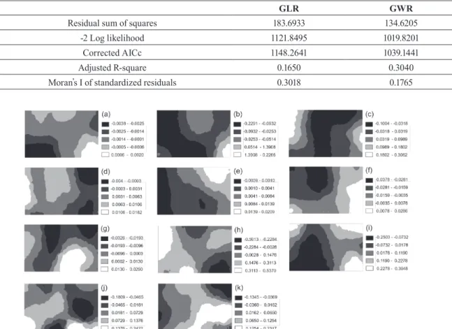
Landslides are major natural geological hazards that result in a large amount of property damage each year, with both direct and indirect costs. Many researchers have produced landslide susceptibility maps using various techniques over the last few decades. This paper presents the landslide susceptibility results from the geographically weighted regression model using remote sensing and geographic information system data for landslide susceptibility in the Inje area of South Korea. Landslide locations were identified from aerial photographs. The eleven landslide-related factors were calculated and extracted from the spatial database and used to analyze landslide susceptibility. Compared with the global logistic regression model, the Akaike Information Criteria was improved by 109.12, the adjusted R-squared was improved from 0.165 to 0.304, and the Moran’s I index of this analysis was improved from 0.4258 to 0.0553. The comparisons of susceptibility obtained from the models show that geographically weighted regression has higher predictive performance.

Keywords : Landslide, Landslide Susceptibility Map, Geographically Weighted Regression, Logistic Regression Model

579 ISSN 1598-4850(Print) ISSN 2288-260X(Online) Original article

Received 2015. 12. 01, Revised 2015. 12. 22, Accepted 2015. 12. 26

1) Member, Dept. of Spatial Information Engineering, Pukyong National University (E-mail: [email protected])

2) Corresponding Author, Member, Dept. of Spatial Information Engineering, Pukyong National University (E-mail: [email protected])

This is an Open Access article distributed under the terms of the Creative Commons Attribution Non-Commercial License (http://

creativecommons.org/licenses/by-nc/3.0) which permits unrestricted non-commercial use, distribution, and reproduction in any medium, provided the original work is properly cited.

1. Introduction

Over the last decade, natural disasters such as hurricanes, earthquakes, extreme erosion, tsunamis, and landslides have increased sharply. Because of increasing threats from these phenomena, national and local government agencies have expressed concern for human injuries and economic loss (Yilmaz, 2009). Landslides, which account for 4.4% of natural disasters around the world, have increased rapidly in frequency and cause significant damage (1990-2009) (Akgun et al., 2008; Vos et al., 2010; Park et al., 2013). This trend will continue in the coming decades, as regional precipitation, deforestation, urbanization, and development increase (Schuster, 1996).

Under these circumstances, interest in landslide assessment

has grown significantly among experts in various fields, such as engineers, geologists, planners, local administrators, and decision makers (Ercanoglu and Gokceoglu, 2004).

Assessment and management of landslide damage can be aided by thematic mapping, with the following steps: 1.

Landslide inventory maps; 2. Landslide susceptibility maps;

3. Landslide hazard maps; and 4. Landslide risk maps (Kamp et al., 2008). Among these maps, the production of a landslide susceptibility map in the early stage of the assessment process is of crucial importance.

Landslide susceptibility maps have been drawn using various methods across numerous research studies. The methods are divided into qualitative and quantitative.

Currently, quantitative techniques are widely used, aided

by the technological development of GIS (Geographical

(2)

580

Information Systems), which provide a powerful tool for managing and manipulating spatial data. Quantitative techniques are based on numerical expressions of the relationships between controlling factors and landslides (Aleotti and Chowdhury, 1999). Quantitative techniques are divided into deterministic and statistical methods (either bivariate or multivariate), and the majority of researchers prefer the GLR (Global Logistic Regression) model, a statistical method (Ayalew and Yamagishi, 2005; Bai et al., 2010; Bui et al., 2011; Chauhan et al., 2010; Chen and Wang, 2007; Falaschi et al., 2009; Xu et al., 2013).

However, the GLR model cannot take into account the spatial dependence or autocorrelation characteristics of observational data (Erener and Düzgün, 2010). This reduces the efficiency of estimated parameters when evaluating landslide susceptibility. Therefore, the GWR (Geographically Weighted Regression) has been introduced as a method that incorporates spatial variation (Feuillet et al., 2014). Because the GWR model uses a regression model, the advantages of existing models can be applied, and different factors can be estimated for respective regions. This makes it possible to confirm a spatially heterogeneous pattern that is difficult to grasp with existing models. Additionally, it enables the visualization of spatial interactions among data by mapping the results of the GWR analysis using GIS (Ercanoglu and Gokceoglu, 2004).

The goal of our study is to analyze and quantify improvements in the accuracy and explanatory power of landslide susceptibility compared with a previously used the GLR model when analyzing landslide susceptibility using the GWR. To accomplish this, the Inje region was selected as the research area, as it was subjected to severe landslide damage in 2006. A spatial database of landslide-related factors was compiled using the DEM (Digital Elevation Model) and various thematic maps. The GWR model was analyzed and compared with the GLR model analysis results using conformity-measured values and various diagnostic indices.

2. Study Area

Approximately 81% of the total area of Gangwon-do in the

central eastern region of Korea is composed of mountains.

Most of these mountains have steep and rough terrain with 2 m or less of effective soil depth: suitable conditions for landslides (Im, 2009).Three instances of localized heavy rainfalls occurred in the Gangwon-do area in 2006 (July 11–

13, July 14–20, July 25–29), including Ewiniar, a category 3 typhoon. These rains were regionally concentrated in the Inje, Yangyang, and Pyeongchang areas, with the heaviest rainfall in about 500 years lasting for about 1–6 hours (Lee and Talib, 2005). This caused approximately 160 billion won in property damage and resulted in 40 or more human deaths. According to Kim et al. (2012), landslides occurred in about 400 locations around Inje-eup, Girin-myun, and Nam- myun, Inje-gun. Among these, a survey revealed that Inje- eup experienced the most landslides and the most damage.

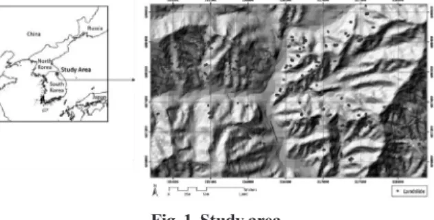
Therefore, the entire area of Inje-eup was selected as the study area for this analysis of landslide susceptibility (Fig. 1).

3. Data set and methodology

3.1. Landslide identification

Accurate identification of landslide locations is critical to analyses of landslide hazards. Field surveys are the most accurate way to identify landslide locations, but terrain and environmental conditions may make it difficult and costly to access these areas as an initial landslide identification method. Remote sensing methods using data such as aerial photos and satellite imagery are more effective due to their lower cost, and are widely used to identify landslide locations (Liangjie et al., 2012).

Landslide locations for this study were identified using aerial photos taken soon after landslide occurrences. Aerial photos taken on 2 August 2006 using the PKNU (Pukyong

Fig. 1. Study area

(3)

A Comparative Analysis of Landslide Susceptibility Assessment by Using Global and Spatial Regression Methods in Inje Area, Korea

581 National University) IV system were used to identify the

locations of landslides that had occurred in the Inje area in July 2006. The collected aerial photos were geometrically corrected using a 1:5,000 digital topographic map and then used to produce orthophotos by creating a mosaic using a DTM (Digital Terrain Model). Landslide locations were digitized by visual interpretation using orthorectified aerial photos.

3.2 Spatial dataset

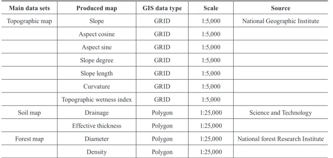
Because landslides result from a combination of various factors such as topology, soil, and forest, these landslide- related factors need to be built into a spatial database for landslide susceptibility analysis. The relevant thematic maps acquired from government were used to construct a spatial database (Table 1). A total of eleven landslide-related factors were compiled into a spatial database with 10×10-m cells relative to the research area using ArcGIS 10.2 software.

The dataset consisted of 232 rows×370 columns, for a total of 85,840 cells, with landslides represented in 446 of the cells.

A total of 446 cells were divided randomly into two groups, training and validation set. 624 cells, accounting for 70%

of the total positive events (landslide affected areas), were randomly selected as the training set. In addition, cells of the

negative events (landslide non-affected areas) were collected with same number of the positive events. The remaining portion of the training set was used as validation set.

3.3. GLR

Regression approaches including linear regression, log- linear regression and logistic regression can be considered a process to extract the coefficients of empirical relationships from observations (Ozdemir and Altural, 2013). The goal of GLR is to find the best-fitting model to describe the relationship between a dichotomous depend variable (the presence or absence of landslides) and several explanatory variables.The explanatory variables may be continuous or discrete (with dummy variables) and do not need a normal frequency distribution (Ayalew and Yamagishi, 2005; Van Den Eeckhaut et al., 2006). Quantitatively, the relationship between depend variable and explanatory variables can be expressed in Eq. (1).

(1)

where, P is the probability of landslide occurrence, ranging between 0 and 1 on an s-shaped curve, and z represents a linear combination of the variables through Eq. (2).

Main data sets Produced map GIS data type Scale Source

Topographic map Slope GRID 1:5,000 National Geographic Institute

  Aspect cosine GRID 1:5,000  

  Aspect sine GRID 1:5,000  

  Slope degree GRID 1:5,000  

  Slope length GRID 1:5,000  

  Curvature GRID 1:5,000  

  Topographic wetness index GRID 1:5,000  

Soil map Drainage Polygon 1:25,000 Science and Technology

  Effective thickness Polygon 1:25,000  

Forest map Diameter Polygon 1:25,000 National forest Research Institute

  Density Polygon 1:25,000  

Table 1. Data type and scale of data used in the study

(4)

Journal of the Korean Society of Surveying, Geodesy, Photogrammetry and Cartography, Vol. 33, No. 6, 579-587, 2015

582

(2)

where,

is the intercept of the model,

are the regression coefficients, and

are the explanatory variables (Youssef et al., 2015). The value z varies from

to

.

A positive sign of the probability represents that the explanatory variables has increased the probability of change, and a negative sign indicates the opposite effect. In addition, maximizing likelihood function is used to obtain the regression coefficients. A coefficient is significant if the tested null hypothesis that the estimated coefficient was zero could be rejected at a 0.05 significance level(Hosmer and Lemeshow, 2000; Kleinbaum and Klein, 2002; Van Den Eeckhaut et al., 2006).

In addition, multicollinearity among the independent variables is tested using the TOL (tolerance) and the VIF (Variance Inflation Factor) to improve the model fitting.

The variables with VIF > 10 and TOL < 0.1 are represented serious multicollinearity between explanatory variables and excluded from the logistic analysis (Hosmer and Lemeshow, 2000; Menard, 2002; Zhu and Huang, 2006).

3.4. GWR

GWR, which is a local modeling technique, aims to capture spatial non-stationarity in the influence of factors on the occurrence of a landslide (Feuillet et al., 2014). The spatial non-stationarity is identified by generating a set of local-specific coefficients, including local R square, local model residuals, local parameter estimates as well as the corresponding t-test values (Fotheringham et al., 2002). The GWR model extends the OLS (Ordinary Regression Squares) regression by allowing regression coefficients to be estimated locally (Feuillet et al., 2014).

The GWR model can be expressed as:

(3)

where

and

are the spatial position of location j,

acts as intercept, and

is the local estimated coefficient for explanatory variables (Su et al., 2012).

The GWR uses kernel bandwidth to determine the spatial

scope of spatialdependence, and then employs distance decay function to weight all the observations within the spatial scope. Because it is assumed that observations near point i have more influence on the estimation of

than observations located farther from i (Feuillet et al., 2014;

Tu and Xia, 2008). The distance decay functions can be calculated by Gaussian and bi-square (Brunsdon et al., 1998;

Fotheringham et al., 2002). In this research, the Gaussian distance decay is used to express the weight function:

(4)

where

is the weight for observation

within the neighborhood of observation

,

represents the distance between observations

and

, and h denotes the kernel bandwidth (Su et al., 2012). The CV (Cross-Validation) and AICc (Akaike Information Criterion) are used to select optimum bandwidth. The AICc is generally more applicable and can be applied in non-Gaussian GWR than CV (Fotheringham et al., 2002; Lloyd, 2010).

Three goodness-of-fit criteria such as deviance, AICc, and the BIC (Bayesian Information Criterion (BIC, also known as the Schwartz criterion) are used to consider both fit and complexity of the model. Lower values of these criteria indicate a more efficient model (Feuillet et al., 2014).

4. Results and Discussion

4.1. Logistic regression

The results of logistic regression model are represented in Table 2.All explanatory variables had the value of VIF

< 10 and TOL > 0.1 respectively. This result indicated that

there was no serious multicollinearity between explanatory

variables. In addition, the significance probability value was

less than 0.01 against all variables except for aspect sine,

topographic wetness index, and soil thickness. This indicates

that the other variables with exception of the above three

variables had statistically significant effects on landslide at

the 5% significance level. From the analysis results, Aspect

sine, slope degree, slope length, soil drainage, soil thickness,

timber diameter, and timber density had positive effects

on landslide occurrence and showed a higher possibility of

(5)

A Comparative Analysis of Landslide Susceptibility Assessment by Using Global and Spatial Regression Methods in Inje Area, Korea

583 landslide. On the other hand, the other variables except for

the above variables had less effect on landslide occurrence.

Timber diameter was the most influential of the landslide- related factors, whereas aspect cosine contributed least to landslide occurrence.

4.2. GWR

Table 3 summarizes the spatially varying coefficients for 714 sample points. All of the eleven explanatory variables have both positive and negative coefficient values although with differences in the portions of both values. This

represented that the constant coefficient estimates in the logistic regression tent to make the spatially non-stationary process of landslide occurrence. The values of slope degree, slope length, and timber density represented over 80% of positive coefficients and the values of elevation and aspect cosine had over 80% of negative coefficients. Also, the values of aspect sin, curvature, topographic wetness index, soil drainage, soil thickness, and timber diameter had apparent divisions of positive and negative results. Such spatially varying coefficients are mostly ignored in the orthodox logistic models.

Variable Coefficient Std. Error t-statistic Sig. Tolerance VIF

Intercept 0.1870 0.1853 1.0089 0.3133 - -

Elevation -0.0015 0.0002 -6.3425 0.0000* 0.6686 1.4956

Aspect cosine -0.0875 0.0223 -3.9188 0.0000* 0.9548 1.0474

Aspect sin 0.01489 0.0222 0.6717 0.5019 0.9584 1.0434

Slope degree 0.0055 0.0021 2.6573 0.0080* 0.6719 1.4883

Slope length 0.0041 0.0014 2.8707 0.0042* 0.3910 2.5576

Curvature -0.0139 0.0058 -2.4156 0.0159* 0.5775 1.7316

Topographic wetness index -0.0044 0.0069 -0.6387 0.5232 0.3915 2.5540

Soil drain 0.0930 0.0421 2.2077 0.0275* 0.5922 1.6887

Soil thickness 0.0261 0.0321 0.8135 0.4161 0.7452 1.3420

Timber diameter 0.0974 0.0220 4.4224 0.0000* 0.7757 1.2891

Timber density 0.0842 0.0220 3.8260 0.0002* 0.7518 1.3302

Table 2. Result of logistic regression

Variable Mean SD Min Max % positive % negative

Intercept -0.0617 0.7054 -2.5460 1.8137 55.83 44.17

Elevation -0.0010 0.0010 -0.0038 0.0021 9.19 90.81

Aspect cosine -0.0646 0.0726 -0.2291 0.2268 17.15 82.85

Aspect sin 0.0225 0.0916 -0.1005 0.3063 51.01 48.99

Slope degree 0.0049 0.0041 -0.0043 0.0183 87.89 12.11

Slope length 0.0042 0.0049 -0.0040 0.0210 90.13 9.87

Curvature -0.0126 0.0152 -0.0379 0.0241 24.33 75.67

Topographic wetness index -0.0033 0.0158 -0.0327 0.0291 36.77 63.23

Soil drain 0.1264 0.2027 -0.5917 0.5371 76.35 23.65

Soil thickness 0.0379 0.1251 -0.2506 0.3952 57.85 42.15

Timber diameter 0.0491 0.0675 -0.1813 0.2424 77.80 22.20

Timber density 0.0670 0.0643 -0.1346 0.2318 86.43 13.57

Table 3. Summary of spatially varying coefficients

(6)

584

4.3. Comparison of model performances The model performance between the GLR and the GWR models was compared using statistical parameters (Table 4).

The GWR model showed significant improvement over the GLR. First, the GWR model had a much better goodness- of-fit than the GLR though the significant decrease of -2 Log likelihood. Second, the AICc index was 1148.2641 in the GLR model and 1049.1441 in the GWR model. If the difference in the AICc index between two models is greater than 4, the model is considered to be improved (Charlton and Fotheringham, 2009). The difference between two models in this study was 109.12, indicating that the conformity of the GWR model was significantly improved. Third, the adjusted R-squared value was 0.165 in the GLR model and 0.304 in the GWR model. Examination of model conformity reveals

whether the general explanation power of the model has improved. Fourth, spatial autocorrelation can be examined more quantitatively using Moran’s I index. Moran’s I index in the GLR model was 0.3018 (p<0.01), indicating the existence of a spatial autocorrelation. However, Moran’s I index in the GWR model was 0.1765 (p<0.01), indicating that the spatial dependence evident in the standardized residual in the GWR model was removed through geographical weighting.

4.4. Spatial varying relationships

The GWR model generates a set of coefficient estimates of explanatory variables for each landslide sample point.

A set of coefficient surfaces based on the sample points with coefficient estimates were generated to reveal the spatially non-stationary relationship between landslide

GLR GWR

Residual sum of squares 183.6933 134.6205

-2 Log likelihood 1121.8495 1019.8201

Corrected AICc 1148.2641 1039.1441

Adjusted R-square 0.1650 0.3040

Moran’s I of standardized residuals 0.3018 0.1765

Table 4. Comparison of GLR and GWR results

Fig. 2. GWR coefficient surfaces of elevation (a), aspect cosine (b), aspect sin (c), slope degree (d), slope length (e), curvature

(f), topographic wetness index (g), soil drainage (h), soil thickness (i), timber diameter (j), and timber density (k)

(7)

A Comparative Analysis of Landslide Susceptibility Assessment by Using Global and Spatial Regression Methods in Inje Area, Korea

585 occurrence and explanatory variables. An IDW (Inverse

Distance Weighted) interpolation was employed to generate coefficient surfaces. Fig.2 represents the coefficient surface of each explanatory variables. As an example, the coefficient of aspect cosine had a negative effect from the result of the GLR model and were mostly negative across the entire study area (Fig.2-b). However, although the coefficient of slope degree obtained from the GLR model had a positive effect on landslide occurrence, this did not hold true for the entire study area. From the result of the GWR model, slope degree had a stronger negative influence in the east of the study area than the west (Fig.2-d).

5. Summary and Conclusions

This study analyzed landslide susceptibility in the Inje region. A spatial database was compiled using landslide- related factors derived from aerial photographs and various thematic maps produced by the government. This study analyzed landslide susceptibility using a GWR model, compared it with the results of the GLR model analysis, and analyzed how much the model has improved. The adjusted R-squared value improved from 0.165 to 0.304 and the AICc, a conformity-measured value of a model, was 1148.2641 in the GLR model and 1039.1441 in the GWR model, for a difference of 109.12. In addition, Moran’s I index for the GWR model was 0.1765 compared to 0.3018 for the GLR model for spatial dependence. From these result, the GWR model has significantly improved the GLR model with better goodness-of-fit. It also reduced the spatial dependence of residuals.

Therefore, the GWR model was more powerful and effective in interpreting relationships between landslide- related factors and landslide occurrence. Especially, character and strength of the relationships identified by the GWR model showed great spatial non-stationarity and scale-dependence. However, the GWR model still presents some disadvantages. The lack of independence among local estimates may led to the failure in valid inferences for the local estimates. In addition, when the number of sample is quite small, the estimated local coefficients can be ineffective or invalid (Su et al., 2012).

References

Akgun, A., Dag, S., and Bulut, F. (2008), Landslide susceptibility mapping for a landslide-prone area (Findikli, NE of Turkey) by likelihood-frequency ratio and weighted linear combination models, Environmental Geology, Vol.

54, pp. 1127-1143.

Aleotti, P. and Chowdhury, R. (1999), Landslide hazard assessment: summary review and new perspectives, Bulletin of Engineering Geology and the Environment, Vol. 58, No. 1, pp. 21-44.

Ayalew, L. and Yamagishi, H. (2005), The application of GIS-based logistic regression for landslide susceptibility mapping in the Kakuda-Yahiko Mountains, Central Japan, Geomorphology, Vol. 65, No. 1, pp. 15-31.

Bai, S.B., Wang, J., Lü, G.N., Zhou, P.G., Hou, S.S., and Xu, S.N. (2010), GIS-based logistic regression for landslide susceptibility mapping of the Zhongxian segment in the Three Gorges area, China, Geomorphology, Vol. 115, No.

1, pp. 23-31.

Brunsdon, C., Fotheringham, A.S., and Charlton, M. (1998), Geographically weighted regression-modelling spatial non-stationarity, Statistician, Vol. 47, No. 3, pp. 31-443.

Bui, D.T., Lofman, O., Revhaug, I., and Dick, O. (2011), Landslide susceptibility analysis in the Hoa Binh province of Vietnam using statistical index and logistic regression, Natural Hazards, Vol. 59, No. 3, pp. 1413-1444.

Charlton, M. and Fotheringham, A. S. (2009), Geographically weighted regression: white paper, National Centre for Geocomputation, Ireland, http://gwr.nuim.ie/downloads/GWR _WhitePaper.pdf (last date accessed: 17 April 2015).

Chauhan, S., Sharma, M., and Arora, M.K. (2010), Landslide susceptibility zonation of the Chamoli region, Garhwal Himalayas, using logistic regression model, Landslides, Vol. 7, No. 4, pp. 411-423.

Chen, Z. and Wang, J. (2007), Landslide hazard mapping using logistic regression model in Mackenzie Valley, Canada, Natural Hazards, Vol. 42, No. 1, pp. 75-89.

Vos, F., Rodriguez, J., Below, R., and Guha-Spair, D. (2010),

Annual Disaster Statistical Review 2009, The Numbers

and Trend, Centre for Research on the Epidemiology of

Disasters (CRED), Brussels, 38p.

(8)

586

Ercanoglu, M. and Gokceoglu, C. (2004), Use of fuzzy relations to produce landslide susceptibility map of a landslide prone area (West Black Sea region, Turkey), Engineering Geology, Vol. 75, No. 3, pp. 229-250.

Erener, A. and Düzgün, H.S.B. (2010), Improvement of statistical landslide susceptibility mapping by using spatial and global regression methods in the case of More and Romsdal (Norway), Landslides, Vol. 7, No. 1, pp. 55-68.

Falaschi, F., Giacomelli, F., Federici, P.R., Puccinelli, A., Avanzi, G.A., Pochini, A., and Robolini, A. (2009), Logistic regression versus artificial neural networks:

landslide susceptibility evaluation in a sample area of the Serchio River valley, Italy, Natural Hazards, Vol. 50, No.

3, pp. 551-569.

Feuillet, T., Coquin, J., Mercier, D., Cossart, E., Decaulne, A., and Jónsson, H.P. (2014), Focusing on the spatial non- stationarity of landslide predisposing factors in northern Iceland Do paraglacial factors vary over space?, Progress in Physical Geography, 0309133314528944.

Fotheringham, A.S., Brunsdon, C., and Charlton, M.E.

(2002), Geographically Weighted Regression: The Analysis of Spatially Varying Relationships. New York:

Wiley.

Hosmer, D.W. and Lemeshow, S. (2000), Applied Logistic Regression. New York: Wiley.

Im, O. (2009), A Study on Characteristics of Landslides and Restoration Works in Damaged Area by Heavy Rainfall- focused on Hongcheon Area in Gangwondo, Master’s thesis, Kangwon University, Korea, 77p. (in Korean with English abstract)

Kamp, U., Growley, B., Khattak, G.A., and Owen, L.A.

(2008), GIS-based landslide susceptibility mapping for the 2005 Kashmir earthquake region, Geomorphology, Vol.

101, pp. 631-642.

Kim, K., Gyoo, G., Yoon, H., Lee, C., Won, M., Lee, B., Woo, C., Kim, S., and Lee, M. (2012), 2011 Forest Disaster White Paper, No. 11-140037-000524-01, Korea Forest Research Institute, Seoul, 29p.

Kleinbaum, D.G. and Klein, M. (2002), Logistic Regression, a Self-learning Text, 2nd ed., New York: Springer.

Lee, S. and Talib, J.A. (2005), Probabilistic landslide susceptibility and factor effect analysis, Environmental

Geology, Vol. 47, No. 7, pp. 982-990.

Liangjie, W., Kazuhide, S., and Shuji, M. (2012), GIS-based landslide susceptibility mapping using logistic regression method with LiDAR data in natural slopes, Disaster Advances, Vol. 5, No. 4, pp. 258-263.

Lloyd, C.D. (2010), Local models for spatial analysis, CRC Press.

Menard, S. (2002), Applied Logistic Regression Analysis, SAGE University Paper. p. 111.

Ozdemir, A. and Altural, T. (2013), A comparative study of frequency ratio, weights of evidence and logistic regression methods for landslide susceptibility mapping:

Sultan Mountains, SW Turkey, Journal of Asian Earth Sciences, Vol. 64, pp. 180-197.

Park, S., Choi, C., Kim, B., and Kim, J. (2013), Landslide susceptibility mapping using frequency ratio, analytic hierarchy process, logistic regression, and artificial neural network methods at the Inje area, Korea, Environmental Earth Sciences, Vol. 68, No. 5, pp. 1443-1464.

Schuster, R. (1996), Socioeconomic significance of landslides, In: Turner A.K., Schuster R.L. (eds.) Landslides:

Investigation and Mitigation, Special Report, National Academic Press Washington, DC, 247, pp 12-36.

Su, S., Xiao, R., and Zhang, Y. (2012), Multi-scale analysis of spatially varying relationships between agricultural landscape patterns and urbanization using geographically weighted regression, Applied Geography, Vol. 32, No. 2, pp. 360-375.

Tu, J. and Xia, Z. (2008), Examining spatially varying relationships between land use and water quality using geographically weighted regression I: model design and evaluation, Science of the Total Environment, Vol. 407, pp.

358-378.

Van Den Eeckhaut, M., Vanwalleghem, T., Poesen, J., Govers, G., Verstraeten, G., and Vandekerckhove, L. (2006), Prediction of landslide susceptibility using rare events logistic regression: a case-study in the Flemish Ardennes, Belgium, Geomorphology, Vol. 76, pp. 392-410.

Xu, C., Xu, X., Dai, F., Wu, Z., He, H., Shi, F., Wu, X., and

Xu, S. (2013), Application of an incomplete landslide

inventory, logistic regression model and its validation for

landslide susceptibility mapping related to the May 12,

(9)

A Comparative Analysis of Landslide Susceptibility Assessment by Using Global and Spatial Regression Methods in Inje Area, Korea

587 2008 Wenchuan earthquake of China, Natural Hazards,

Vol. 68, No. 2, pp. 883-900.

Yilmaz, I. (2009), Landslide susceptibility mapping using frequency ratio, logistic regression, artificial neural networks and their comparison: a case study from Kat landslides (Tokat-Turkey), Computers & Geosciences, Vol.

35, No. 6, pp. 1125-1138.

Youssef, A.M., Pradhan, B., Pourghasemi, H.R., and Abdullahi, S. (2015), Landslide susceptibility assessment at Wadi Jawrah Basin, Jizan region, Saudi Arabia using two bivariate models in GIS. Geosciences Journal, pp.

1-21.

Zhu, L. and Huang, J.F. (2006), GIS-based logistic regression

method for landslide susceptibility mapping in regional

scale, Journal of Zhejiang University Science A, Vol. 7,

No. 12, pp. 2007-2017.

(10)

수치

Fig. 1. Study area
Table 1. Data type and scale of data used in the study
Table 2. Result of logistic regression
Table 4. Comparison of GLR and GWR results

참조

관련 문서