A Comparative Study of the Frequency Ratio and Evidential Belief Function Models for Landslide Susceptibility Mapping

(1)

https://doi.org/10.7848/ksgpc.2016.34.6.597

A Comparative Study of the Frequency Ratio and Evidential Belief Function Models for Landslide Susceptibility

Mapping

Yoo, Youngwoo

¹⁾

· Baek, Taekyung

²⁾

· Kim, Jinsoo

³⁾

· Park, Soyoung

⁴⁾

Abstract

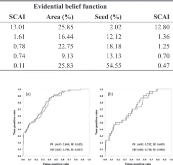
The goal of this study was to analyze landslide susceptibility using two different models and compare the results. For this purpose, a landslide inventory map was produced from a field survey, and the inventory was divided into two groups for training and validation, respectively. Sixteen landslide conditioning factors were considered. The relationships between landslide occurrence and landslide conditioning factors were analyzed using the FR (Frequency Ratio) and EBF (Evidential Belief Function) models. The LSI (Landslide Susceptibility Index) maps that were produced were validated using the ROC (Relative Operating Characteristics) curve and the SCAI (Seed Cell Area Index). The AUC (Area under the ROC Curve) values of the FR and EBF LSI maps were 80.6% and 79.5%, with prediction accuracies of 72.7% and 71.8%, respectively. Additionally, in the low and very low susceptibility zones, the FR LSI map had higher SCAI values compared to the EBF LSI map, as high as 0.47%p. These results indicate that both models were reasonably accurate, however that the FR LSI map had a slightly higher accuracy for landslide susceptibility mapping in the study area.

Keywords : Evidential Belief Function, Frequency Ratio, Landslide Susceptibility, Landslide Susceptibility Index, Landslide Susceptibility Mapping

Original article

Received 2016. 11. 25, Revised 2016. 12. 19, Accepted 2016. 12. 28

1) Dept. of Urban Engineering, Dongeui University (E-mail: [email protected]) 2) Dept. of Urban Engineering, Dongeui University (E-mail: [email protected])

3) Member, Dep. of Spatial Information Engineering, Pukyong National University (E-mail: [email protected])

4) Corresponding Author, Member, Graduate School of Earth Environmental Hazard System, Pukyong National University (E-mail: [email protected]) This is an Open Access article distributed under the terms of the Creative Commons Attribution Non-Commercial License (http://

creativecommons.org/licenses/by-nc/3.0) which permits unrestricted non-commercial use, distribution, and reproduction in any medium,

1. Introduction

Landslides, defined as the movement of a mass of rock or debris, are significant natural hazards. They are caused by various causes, including rainfall, bedrock conditions, vegetation surcharge, groundwater, and human activities (Cruden, 1991; Gerath et al., 1997). Each year, landslides cause casualties and economic losses amounting to more than 100,000 deaths and injuries and more than one billion USD (Schuster, 1996). In Korea, approximately 70% of the

land is mountainous, consisting mainly of granite gneiss. It rains frequently in the region, and typhoons also bring strong winds and heavy rains during the rainy season. Under these circumstances, landslide occurrences have recently become larger and more frequent (KOSIS, 2016).

Landslide susceptibility mapping has become an essential

part of the strategies applied to mitigate and manage

landslide hazards eﬃciently and eﬀectively. To illustrate

for planners which sites (either rural or urban) are suitable

for development, maps of susceptibility to landslides divide

(2)

areas of land into sections, diﬀerentiated by the degree (potential or actual) to which they constitute a landslide hazard (Pourghasemi et al., 2013). In recent years, various models incorporating GIS (Geographic Information System) and remote sensing data have been used to assess landslide susceptibility. GIS models yield advantages in multisource data analysis, particularly when heterogenic or uncertain data is involved (Bui et al., 2012).

Among such models, the FR (Frequency Ratio) model has been used widely to simplify assessment (Lee and Sambath, 2006; Mohammedy et al., 2012). In addition, LR (Logistic Regression), a statistical model, has also been used (Akgun, 2012; Süzen and Doyuran, 2004; Yalcin et al., 2011). Data mining models such as ANN (Artificial Neural Network) (Ermini et al., 2005; Yilmaz, 2009), decision trees (Pradhan, 2013; Saito et al., 2009), and fuzzy logic (Bui et al., 2012) models have similarly been used to assess landslide susceptibility. More recently, the EBF (Evidential Belief Function) (Lee et al., 2013; Pourghasemi and Kerle, 2016), the index of entropy (Hong et al., 2016), and support vector machine (Su et al., 2015) models have been applied.

A number of models have been suggested and implemented, but there is still no agreement on the best model and technique for mapping landslide susceptibility (Wang and Sassa, 2005). Therefore, various models should be applied in a study area and the results should be compared. In Korea, the FR, LR, and ANN have been used widely to analyze landslide susceptibility (Jang et al., 2004; Lee et al., 2012;

Oh, 2010; Yeon, 2011). However, few studies have compared the results from the various models. Additionally, the EBF model has occasionally been used for landslide susceptibility mapping. The eﬃcacy and applicability of the EBF model can be assessed through comparison with the FR model, which is also a bivariate statistical model and its accuracy has been confirmed by many studies. This study assessed and compared the results of LSMs (Landslide Susceptibility Maps) derived using the FR and EBF models and GIS data for spatial prediction of landslide hazards.

2. Study Area

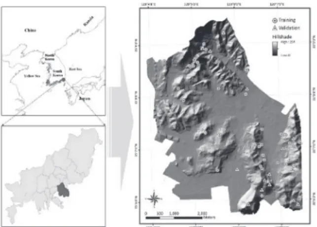
The study area is located at Nam-gu, in the southern part

of Busan Metropolitan City, South Korea. The area covers approximately 25 km

²

, excluding some areas where spatial data could not be collected. It lies between the latitudes of 35°6′ to 35°9′ N and the longitudes of 129°4′ to 129°7′ E (Fig. 1). The annual average temperature is 14.8°C and the annual average precipitation is 1535 mm (from 2000 to 2009;

BMCN, 2016). Heavy rain was concentrated in Busan in July 2009. The heaviest precipitation (average: 260 mm, rate: 86 mm/h) was recorded on July 16, 2009. According to the Busan Metropolitan City Hall, many roads, homes, and stores were ﬂooded and destroyed by the heavy rain. Additionally, 142 landslides occurred throughout Busan Metropolitan City; of these, 27.9% occurred within the study area. This study was based on the landslides that occurred in Nam-gu in July 2009.

3. Data and Methodology

3.1 Landslide inventory map

A landslide inventory map, which is essential for analyzing landslide susceptibility, can be produced by various methods, such as aerial photographs, satellite imagery, airborne LiDAR, and field surveying. In this study, a landslide inventory map was produced using the results of a comprehensive field survey performed by the Busan Metropolitan City Hall. From the 99 landslides identified, 69 (70%) locations were chosen randomly for model training and the remaining 30 (30%) locations were used for model validation (Fig. 1).

Fig. 1. Study area location map with hillshading and

landslide inventory

(3)

3.2 Landslide conditioning factors

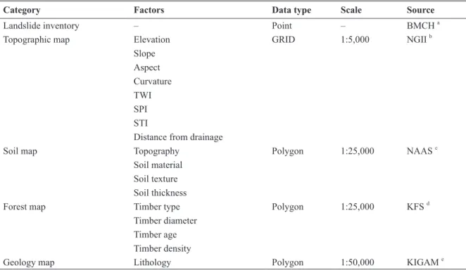
Landslide conditioning factors were collected and compiled from relevant thematic maps acquired from the Korean government. In total, 16 factors were used, and these were divided into three groups (Table 1 and Fig. 2).

The topographic factors, including elevation, slope, aspect, curvature, TWI (Topographic Wetness Index), SPI (Stream Power Index), STI (Sediment Transport Index), and distance from drainage, were derived from a DEM (Digital Elevation Model) produced using 1:5,000-scale topographic maps with ArcGIS software v. 10.2 (ESRI, Redlands, CA). Among these factors, those related to the spatial variation of hydrological conditions, including TWI, SPI, and STI, were produced based on specific catchment areas and a slope map. The amount of water accumulated was measured using the TWI.

Discharge was assumed to be proportional to the catchment area of relevance, allowing the SPI to measure the power to erode of the water ﬂow. The STI measures the overland ﬂow’s capacity to transport sediments (Pourghasemi et al., 2013).

These factors were calculated based on the formulas given

by Beven and Kirkby (1979), Moore et al., (1991), and Moore and Wilson (1992), respectively, as follows:

TWI = ln (

_{tan 𝛽𝛽}^𝑎𝑎

) (1) SPI = 𝐴𝐴

_𝑠𝑠

× 𝑡𝑡𝑡𝑡𝑡𝑡𝑡𝑡 (2)

STI = �

_22.13^𝐴𝐴^𝑠𝑠

�

^0.6

�

_0.0896^{𝑠𝑠𝑠𝑠𝑠𝑠𝛽𝛽}

�

^1.3

(3) 𝑡𝑡

𝐵𝐵𝐵𝐵𝐵𝐵

𝑐𝑐_{𝑖𝑖𝑖𝑖}

=

𝑁𝑁�𝐶𝐶𝑖𝑖𝑖𝑖∩𝐷𝐷�/𝑁𝑁(𝐶𝐶𝑖𝑖𝑖𝑖) 𝑁𝑁(𝐷𝐷)−𝑁𝑁�𝐶𝐶𝑖𝑖𝑖𝑖∩𝐷𝐷�/𝑁𝑁(𝑇𝑇)−𝑁𝑁(𝐶𝐶𝑖𝑖𝑖𝑖)

∑ 𝑁𝑁�𝐶𝐶𝑖𝑖𝑖𝑖∩𝐷𝐷�/𝑁𝑁(𝐶𝐶𝑖𝑖𝑖𝑖) 𝑁𝑁(𝐷𝐷)−𝑁𝑁�𝐶𝐶𝑖𝑖𝑖𝑖∩𝐷𝐷�/𝑁𝑁(𝑇𝑇)−𝑁𝑁(𝐶𝐶𝑖𝑖𝑖𝑖) 𝑚𝑚𝑖𝑖=1

(4)

𝐷𝐷𝐷𝐷𝐷𝐷

=

𝑁𝑁�𝐶𝐶𝑖𝑖𝑖𝑖∩𝐷𝐷�/𝑁𝑁(𝐶𝐶𝑖𝑖𝑖𝑖)

𝑁𝑁(𝑇𝑇)−𝑁𝑁(𝐷𝐷)−[𝑁𝑁�𝐶𝐶𝑖𝑖𝑖𝑖�−𝑁𝑁�𝐶𝐶𝑖𝑖𝑖𝑖∩𝐷𝐷�]/𝑁𝑁(𝑇𝑇)−𝑁𝑁(𝐶𝐶𝑖𝑖𝑖𝑖)

∑ 𝑁𝑁�𝐶𝐶𝑖𝑖𝑖𝑖∩𝐷𝐷�/𝑁𝑁(𝐶𝐶𝑖𝑖𝑖𝑖)

𝑁𝑁(𝑇𝑇)−𝑁𝑁(𝐷𝐷)−[𝑁𝑁�𝐶𝐶𝑖𝑖𝑖𝑖�−𝑁𝑁�𝐶𝐶𝑖𝑖𝑖𝑖∩𝐷𝐷�]/𝑁𝑁(𝑇𝑇)−𝑁𝑁(𝐶𝐶𝑖𝑖𝑖𝑖) 𝑚𝑚𝑖𝑖=1

(5)

Unc = �1 − (𝐵𝐵𝐵𝐵𝐵𝐵

𝐶𝐶_{𝑖𝑖𝑖𝑖}

) − (𝐷𝐷𝐷𝐷𝐷𝐷

)� (6)

Pls = �1 − (𝐷𝐷𝐷𝐷𝐷𝐷

)� (7) where 𝑁𝑁�𝐶𝐶

_{𝑠𝑠𝑖𝑖}

∩ 𝐷𝐷� is the density of landslides given in D, 𝑁𝑁(𝐶𝐶

𝑠𝑠𝑖𝑖

)

(1)

TWI = ln (

) (1) SPI = 𝐴𝐴

𝑠𝑠

× 𝑡𝑡𝑡𝑡𝑡𝑡𝑡𝑡 (2)

STI = �

_22.13^𝐴𝐴^𝑠𝑠

�

^0.6

�

^1.3

(3) 𝑡𝑡

𝐵𝐵𝐵𝐵𝐵𝐵

=

(4)

𝐷𝐷𝐷𝐷𝐷𝐷

𝑐𝑐𝑖𝑖𝑖𝑖

=

(5)

Unc = �1 − (𝐵𝐵𝐵𝐵𝐵𝐵

) − (𝐷𝐷𝐷𝐷𝐷𝐷

)� (6) Pls = �1 − (𝐷𝐷𝐷𝐷𝐷𝐷

_𝐶𝐶_{𝑖𝑖𝑖𝑖}

)� (7) where 𝑁𝑁�𝐶𝐶

𝑠𝑠𝑖𝑖

∩ 𝐷𝐷� is the density of landslides given in D, 𝑁𝑁(𝐶𝐶

𝑠𝑠𝑖𝑖

)

(2)

TWI = ln (

) (1) SPI = 𝐴𝐴

𝑠𝑠

× 𝑡𝑡𝑡𝑡𝑡𝑡𝑡𝑡 (2)

STI = �

_22.13^𝐴𝐴^𝑠𝑠

�

^0.6

�

^1.3

(3) 𝑡𝑡

𝐵𝐵𝐵𝐵𝐵𝐵

=

(4)

𝐷𝐷𝐷𝐷𝐷𝐷

=

(5)

Unc = �1 − (𝐵𝐵𝐵𝐵𝐵𝐵

) − (𝐷𝐷𝐷𝐷𝐷𝐷

)� (6)

Pls = �1 − (𝐷𝐷𝐷𝐷𝐷𝐷

)� (7) where 𝑁𝑁�𝐶𝐶

_{𝑠𝑠𝑖𝑖}

∩ 𝐷𝐷� is the density of landslides given in D, 𝑁𝑁(𝐶𝐶

𝑠𝑠𝑖𝑖

)

(3)

where

TWI = ln ( _{tan 𝛽𝛽} ^𝑎𝑎 ) (1)

SPI = 𝐴𝐴 𝑠𝑠 × 𝑡𝑡𝑡𝑡𝑡𝑡𝑡𝑡 (2)

STI = � _22.13 ^𝐴𝐴

^𝑠𝑠

� ^0.6 � _0.0896 ^{𝑠𝑠𝑠𝑠𝑠𝑠𝛽𝛽} � ^1.3 (3) 𝑡𝑡

𝐵𝐵𝐵𝐵𝐵𝐵 𝑐𝑐

_{𝑖𝑖𝑖𝑖}

=

∑

𝑁𝑁�𝐶𝐶𝑖𝑖𝑖𝑖∩𝐷𝐷�/𝑁𝑁(𝐶𝐶𝑖𝑖𝑖𝑖) 𝑁𝑁(𝐷𝐷)−𝑁𝑁�𝐶𝐶𝑖𝑖𝑖𝑖∩𝐷𝐷�/𝑁𝑁(𝑇𝑇)−𝑁𝑁(𝐶𝐶𝑖𝑖𝑖𝑖) 𝑚𝑚𝑖𝑖=1

(4)

𝐷𝐷𝐷𝐷𝐷𝐷 𝑐𝑐

𝑖𝑖𝑖𝑖

=

∑

(5)

Unc = �1 − (𝐵𝐵𝐵𝐵𝐵𝐵 𝐶𝐶

_{𝑖𝑖𝑖𝑖}

) − (𝐷𝐷𝐷𝐷𝐷𝐷 𝐶𝐶

_{𝑖𝑖𝑖𝑖}

)� (6)

Pls = �1 − (𝐷𝐷𝐷𝐷𝐷𝐷 𝐶𝐶

_{𝑖𝑖𝑖𝑖}

)� (7) where 𝑁𝑁�𝐶𝐶 _{𝑠𝑠𝑖𝑖} ∩ 𝐷𝐷� is the density of landslides given in D, 𝑁𝑁(𝐶𝐶 𝑠𝑠𝑖𝑖 )

is the upslope contributing area, A

_s

is the specific catchment’s area, and β is the local slope gradient measured in degrees.

Soil factors, including topography, soil material, soil texture, and soil thickness, were constructed using a 1:25,000-scale soil map. Forest factors, including timber type, timber diameter, timber age, and timber density, were produced from a 1:25,000-scale forest map. Additionally, lithology was extracted from a 1:50,000-scale geologic map.

The 16 landslide conditioning factors that were produced were converted into 10-m-resolution raster grids. The

Table 1. Data layers used to analyze landslide susceptibility

Category Factors Data type Scale Source

Landslide inventory – Point – BMCH

^a

Topographic map Elevation GRID 1:5,000 NGII

^b

Slope Aspect Curvature TWI SPI STI

Distance from drainage

Soil map Topography Polygon 1:25,000 NAAS

^c

Soil material Soil texture Soil thickness

Forest map Timber type Polygon 1:25,000 KFS

^d

Timber diameter Timber age Timber density

Geology map Lithology Polygon 1:50,000 KIGAM

^e

a

Busan Metropolitan City Hall;

^b

National Geographic Information Institute;

^c

National Academy of Agriculture Science;

d

Korea Forest Service;

^e

Korea Institute of Geoscience and Mineral Resources

(4)

dimensions of the study area grid were 704 rows by 555 columns, so the total number of cells was therefore 390,720.

4. Results and Discussion

4.1 Landslide susceptibility mapping 4.1.1 FR

In general, the locations and frequencies of landslides are assumed to depend on a number of factors that create conditions under which landslides can occur. Future landslides are predicted to occur when conditions are the same as those that prevailed when they occurred in the past (Lee and Pradhan, 2007). The FR correlates an area of past landslides with the total area under consideration. Ratios higher than 1 indicate that occurrence and conditioning factors correlate closely, whereas values <1 indicate that the correlation is weaker (Akgun, 2012).

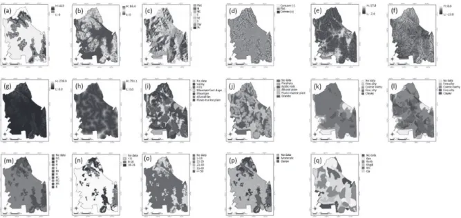
FR values were calculated for each range or category of the 16 landslide conditioning factors (Table 2). FR values increased with increasing values of elevation, and were highest for the >318 m class (3.782). With regards to slope, the 3.0–7.5˚ and >23.9˚ ranges had the highest correlations with landslide occurrence. Most landslides occurred on

east- and southwest-facing slopes, with FR values of 2.540 and 2.014, respectively. Convex areas had a higher FR value (1.375) than concave areas (1.298). For the case of TWI, the

<3.2 classes, excluding the -5.2–0.4 class, had FR values

>1.0. Among these classes, the 1.6–2.4 class had the highest FR value (1.607). The FR values of SPI mostly increased with increasing SPI values. The >2.1 class had the highest correlation with landslide occurrence. Similarly, for STI, the

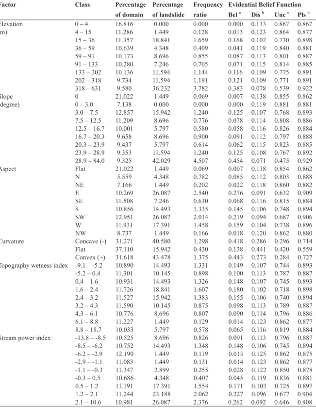
>35.0 class had the highest FR value at 3.541. With regards to distance from drainage, the distance classes of 1–28.4 m and 113.4–158.0 m had high FR values of 1.573 and 2.717, respectively. Mountain foot slope and mountain were more suitable for landslide occurrence. With regards to soil material, most landslides occurred in the porphyry and acidic rock classes. The fine silty and clayey classes showed high correlations, with values of 1.271 and 1.309, respectively. The soil thickness class of 20–50 cm had a FR value of 1.465. Most landslides occurred in Pine (D) and Pinus rigida (PR) forests.

Additionally, the 6–16 cm, 21–40 years, and dense classes had the highest correlations with landslide occurrence. With regards to geology, the andesite (Kan) and volcanic breccia (Kanb) classes had FR values of 3.061 and 1.044, respectively (Table 2).

Fig. 2. Landslide conditioning factors: (a) elevation, (b) slope, (c) aspect, (d) curvature, (e) TWI, (f) SPI, (g) STI, (h) distance from drainage, (i) soil topography, (j) soil material, (k) soil texture, (l) soil thickness, (m) timber type,

(n) timber diameter, (o) timber age, (p) timber density, and (q) lithology

(5)

Table 2. Spatial relationship between each landslide conditioning factor and landslides using the frequency ratio and the evidential belief function

Factor Class Percentage Percentage Frequency Evidential Belief Function

of domain of landslide ratio Bel

^a

Dis

^b

Unc

^c

Pls

^d

Elevation 0 – 4 16.816 0.000 0.000 0.000 0.133 0.867 0.867

(m) 4 – 15 11.286 1.449 0.128 0.013 0.123 0.864 0.877

15 – 36 11.357 18.841 1.659 0.168 0.102 0.730 0.898

36 – 59 10.639 4.348 0.409 0.041 0.119 0.840 0.881

59 – 91 10.173 8.696 0.855 0.087 0.113 0.801 0.887

91 – 133 10.280 7.246 0.705 0.071 0.115 0.814 0.885

133 – 202 10.136 11.594 1.144 0.116 0.109 0.775 0.891

202 – 318 9.734 11.594 1.191 0.121 0.109 0.771 0.891

318 – 631 9.580 36.232 3.782 0.383 0.078 0.539 0.922

Slope 0 21.022 1.449 0.069 0.007 0.138 0.855 0.862

(degree) 0 – 3.0 7.138 0.000 0.000 0.000 0.119 0.881 0.881

3.0 – 7.5 12.857 15.942 1.240 0.125 0.107 0.768 0.893

7.5 – 12.5 11.209 8.696 0.776 0.078 0.114 0.808 0.886

12.5 – 16.7 10.001 5.797 0.580 0.058 0.116 0.826 0.884

16.7 – 20.3 9.658 8.696 0.900 0.091 0.112 0.797 0.888

20.3 – 23.9 9.437 5.797 0.614 0.062 0.115 0.823 0.885

23.9 – 28.9 9.353 11.594 1.240 0.125 0.108 0.767 0.892

28.9 – 84.0 9.325 42.029 4.507 0.454 0.071 0.475 0.929

Aspect Flat 21.022 1.449 0.069 0.007 0.138 0.854 0.862

N 5.559 4.348 0.782 0.085 0.112 0.803 0.888

NE 7.166 1.449 0.202 0.022 0.118 0.860 0.882

E 10.269 26.087 2.540 0.276 0.091 0.632 0.909

SE 11.508 7.246 0.630 0.068 0.116 0.815 0.884

S 10.856 14.493 1.335 0.145 0.106 0.748 0.894

SW 12.951 26.087 2.014 0.219 0.094 0.687 0.906

W 11.931 17.391 1.458 0.159 0.104 0.738 0.896

NW 8.737 1.449 0.166 0.018 0.120 0.862 0.880

Curvature Concave (-) 31.271 40.580 1.298 0.418 0.286 0.296 0.714

Flat 37.110 15.942 0.430 0.138 0.441 0.420 0.559

Convex (+) 31.618 43.478 1.375 0.443 0.273 0.284 0.727

Topography wetness index -9.1 – -5.2 10.890 14.493 1.331 0.149 0.107 0.744 0.893

-5.2 – 0.4 11.301 10.145 0.898 0.100 0.113 0.787 0.887

0.4 – 1.6 10.931 14.493 1.326 0.148 0.107 0.745 0.893

1.6 – 2.4 11.726 18.841 1.607 0.180 0.102 0.718 0.898

2.4 – 3.2 11.527 15.942 1.383 0.155 0.106 0.740 0.894

3.2 – 4.3 11.590 10.145 0.875 0.098 0.113 0.789 0.887

4.3 – 6.1 10.776 8.696 0.807 0.090 0.114 0.796 0.886

6.1 – 8.8 11.227 1.449 0.129 0.014 0.123 0.862 0.877

8.8 – 18.7 10.033 5.797 0.578 0.065 0.116 0.819 0.884

Stream power index -13.8 – -8.5 10.525 8.696 0.826 0.091 0.113 0.796 0.887

-8.5 – -6.2 10.752 14.493 1.348 0.148 0.106 0.745 0.894

-6.2 – -2.9 12.190 1.449 0.119 0.013 0.125 0.862 0.875

-2.9 – -1.1 11.083 1.449 0.131 0.014 0.123 0.862 0.877

-1.1 – -0.3 11.347 2.899 0.255 0.028 0.122 0.850 0.878

-0.3 – 0.5 10.686 4.348 0.407 0.045 0.119 0.836 0.881

0.5 – 1.2 11.191 17.391 1.554 0.171 0.103 0.725 0.897

1.2 – 2.1 11.244 23.188 2.062 0.227 0.096 0.677 0.904

2.1 – 10.6 10.981 26.087 2.376 0.262 0.092 0.646 0.908

(6)

Table 2. (continued)

Factor Class Percentage Percentage Frequency Evidential Belief Function of domain of landslide ratio

Bel

^a

Dis

^b

Unc

^c

Pls

^d

Sediment transport index 0 40.491 24.638 0.608 0.047 0.139 0.814 0.861

0 – 2.7 14.073 1.449 0.103 0.008 0.126 0.866 0.874

2.7 – 5.4 7.075 1.449 0.205 0.016 0.116 0.868 0.884

5.4 – 8.1 7.819 10.145 1.297 0.100 0.107 0.793 0.893

8.1 – 13.5 6.518 7.246 1.112 0.086 0.109 0.805 0.891

13.5 – 18.8 7.145 5.797 0.811 0.063 0.111 0.826 0.889

18.8 – 24.2 5.491 13.043 2.376 0.184 0.101 0.715 0.899

24.2 – 35.0 6.067 17.391 2.866 0.222 0.097 0.682 0.903

35.0 – 686.3 5.321 18.841 3.541 0.274 0.094 0.632 0.906

Distance from drainage 0 – 28.4 11.058 17.391 1.573 0.178 0.103 0.718 0.897

(m) 28.4 – 68.9 10.255 7.246 0.707 0.080 0.115 0.805 0.885

68.9 – 113.4 12.418 5.797 0.467 0.053 0.120 0.828 0.880

113.4 – 158.0 12.266 33.333 2.717 0.308 0.084 0.607 0.916

158.0 – 206.6 10.394 7.246 0.697 0.079 0.115 0.806 0.885

206.6 – 259.3 11.661 7.246 0.621 0.070 0.117 0.813 0.883

259.3 – 324.1 10.824 7.246 0.669 0.076 0.116 0.808 0.884

324.1 – 417.3 10.785 8.696 0.806 0.091 0.114 0.795 0.886

417. 3 – 1029.1 10.339 5.797 0.561 0.064 0.117 0.820 0.883

Soil topography No data 8.999 0.000 0.000 0.000 0.157 0.843 0.843

Valley 0.858 0.000 0.000 0.000 0.145 0.855 0.855

Hills 27.563 23.188 0.841 0.171 0.152 0.677 0.848

Mountain foot slope 23.260 24.638 1.059 0.216 0.141 0.643 0.859

Mountain 18.617 47.826 2.569 0.524 0.092 0.384 0.908

Alluvial fan 6.092 1.449 0.238 0.048 0.150 0.801 0.850

Fluvio-marine plain 14.610 2.899 0.198 0.040 0.163 0.797 0.837

Soil material No data 8.999 0.000 0.000 0.000 0.189 0.811 0.811

Porphyry 44.626 71.014 1.591 0.521 0.090 0.389 0.910

Acidic rock 23.984 24.638 1.027 0.336 0.170 0.493 0.830

Alluvial plain 6.092 1.449 0.238 0.078 0.180 0.742 0.820

Fluvio-marine plain 14.610 2.899 0.198 0.065 0.195 0.740 0.805

Granite 1.689 0.000 0.000 0.000 0.175 0.825 0.825

Soil texture No data 8.999 0.000 0.000 0.000 0.241 0.759 0.759

Fine silty 0.134 0.000 0.000 0.000 0.219 0.781 0.781

Coarse loamy 14.627 2.899 0.198 0.071 0.249 0.680 0.751

Fine silty 70.706 89.855 1.271 0.457 0.076 0.467 0.924

Clayey 5.534 7.246 1.309 0.471 0.215 0.314 0.785

Soil thickness No data 8.999 0.000 0.000 0.000 0.227 0.773 0.773

(cm) < 20 2.376 1.449 0.610 0.199 0.209 0.592 0.791

20 – 50 48.471 71.014 1.465 0.478 0.116 0.406 0.884

50 – 100 32.231 26.087 0.809 0.264 0.226 0.510 0.774

> 100 7.922 1.449 0.183 0.060 0.222 0.719 0.778

Timber type No data 70.320 40.580 0.577 0.044 0.172 0.784 0.828

Retinispora

0.547 0.000 0.000 0.000 0.086 0.914 0.914

Pine 14.192 33.333 2.349 0.180 0.067 0.753 0.933

Deciduous 1.946 1.449 0.745 0.057 0.086 0.857 0.914

Farmland 0.397 0.000 0.000 0.000 0.086 0.914 0.914

Mixed forest 6.470 2.899 0.448 0.034 0.089 0.877 0.911

Non-stocked forest 1.453 0.000 0.000 0.000 0.087 0.913 0.913

Artificial coniferous 0.352 0.000 0.000 0.000 0.086 0.914 0.914

(7)

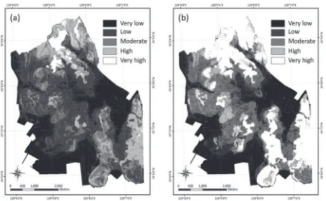
The calculated FR values were summed to calculate the LSI (Landslide Susceptibility Index). The LSI map (hereafter, FR LSI map) was classified into five zones by natural-break classification for ease of visual interpretation: very low, low, moderate, high, and very high landslide susceptibility zones.

These landslide susceptibility zones made up 26.3%, 37.3%, 28.9%, 14.1%, and 3.4% of the study area, respectively.

Approximately 17% of the study area was particularly susceptible to landslide occurrence (Fig. 3a).

4.1.2 EBF

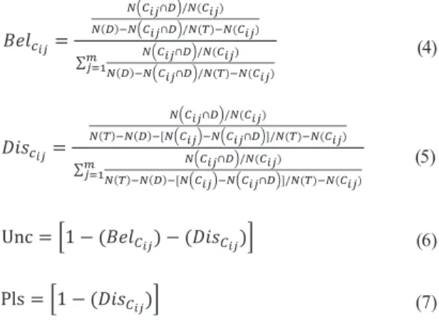
The EBF, which has its roots in Dempster–Shafer theory, is a way to bring together a number of separate items of information (the ‘evidence’) to allow for the calculation of the likelihood (the ‘probability’) that something will happen (the ‘event’) (Tangestani, 2009). There are four important EBF functions: the extent to which something is believed (Bel), the extent to which it is disbelieved (Dis), the degree of uncertainty (Unc), and the degree of plausibility (Pls) (Pourghasemi and Kerle, 2016). The upper and lower probability bounds are Pls and Bel. Unc represents the diﬀerence between belief and plausibility (Awasthi and Chauhan, 2011; Tien et al., 2012). These four functions are calculated as follows:

Table 2. (continued)

a

Believed;

^b

disbelieved;

^c

the degree of uncertainty;

^d

the degree of plausibility

Factor Class Percentage Percentage Frequency Evidential Belief Function of domain of landslide ratio

Bel

^a

Dis

^b

Unc

^c

Pls

^d

Timber type Artificial pine 0.715 0.000 0.000 0.000 0.086 0.914 0.914

Pinus regida

2.443 21.739 8.899 0.684 0.069 0.248 0.931

Left-over area 1.166 0.000 0.000 0.000 0.087 0.913 0.913

Timber diameter No data 73.336 40.580 0.553 0.096 0.459 0.446 0.541

(cm) < 6 1.418 0.000 0.000 0.000 0.209 0.791 0.791

6 – 16 10.577 44.928 4.248 0.734 0.127 0.140 0.873

18 – 28 14.668 14.493 0.988 0.171 0.206 0.623 0.794

Timber age No data 73.336 40.580 0.553 0.066 0.324 0.609 0.676

(years) 1 – 10 1.418 0.000 0.000 0.000 0.148 0.852 0.852

11 – 20 1.112 0.000 0.000 0.000 0.147 0.853 0.853

21 – 30 5.547 36.232 6.531 0.781 0.098 0.120 0.902

31 – 40 18.218 23.188 1.273 0.152 0.137 0.711 0.863

>= 50 0.368 0.000 0.000 0.000 0.146 0.854 0.854

Timber density No data 74.754 40.580 0.543 0.119 0.597 0.284 0.403

Moderate 8.914 7.246 0.813 0.179 0.258 0.563 0.742

Dense 16.332 52.174 3.195 0.702 0.145 0.153 0.855

Geology No data 9.269 0.000 0.000 0.000 0.182 0.818 0.818

Andesite 13.731 42.029 3.061 0.557 0.111 0.332 0.889

Volcanic breccia 27.765 28.986 1.044 0.190 0.163 0.647 0.837

Hornblende granodiorite 4.382 1.449 0.331 0.060 0.171 0.769 0.829

Sedimentary rock 7.125 2.899 0.407 0.074 0.173 0.753 0.827

Alluvium 37.728 24.638 0.653 0.119 0.200 0.681 0.800

Fig. 3. Landslide susceptibility map produced using (a) the frequency ratio and

(b) the evidential belief function

(8)

Journal of the Korean Society of Surveying, Geodesy, Photogrammetry and Cartography, Vol. 34, No. 6, 597-607, 2016

tan 𝛽𝛽

SPI = 𝐴𝐴

𝑠𝑠

× 𝑡𝑡𝑡𝑡𝑡𝑡𝑡𝑡 (2)

STI = �

_22.13^𝐴𝐴^𝑠𝑠

�

^0.6

�

^1.3

(3) 𝑡𝑡

𝐵𝐵𝐵𝐵𝐵𝐵

=

(4)

𝐷𝐷𝐷𝐷𝐷𝐷

=

(5)

Unc = �1 − (𝐵𝐵𝐵𝐵𝐵𝐵

) − (𝐷𝐷𝐷𝐷𝐷𝐷

)� (6) Pls = �1 − (𝐷𝐷𝐷𝐷𝐷𝐷

)� (7) where 𝑁𝑁�𝐶𝐶

_{𝑠𝑠𝑖𝑖}

∩ 𝐷𝐷� is the density of landslides given in D, 𝑁𝑁(𝐶𝐶

_{𝑠𝑠𝑖𝑖}

)

(4) SPI = 𝐴𝐴

𝑠𝑠

× 𝑡𝑡𝑡𝑡𝑡𝑡𝑡𝑡 (2)

STI = �

_22.13^𝐴𝐴^𝑠𝑠

�

^0.6

�

^1.3

(3) 𝑡𝑡

𝐵𝐵𝐵𝐵𝐵𝐵

=

(4)

𝐷𝐷𝐷𝐷𝐷𝐷

=

(5)

Unc = �1 − (𝐵𝐵𝐵𝐵𝐵𝐵

) − (𝐷𝐷𝐷𝐷𝐷𝐷

)� (6)

Pls = �1 − (𝐷𝐷𝐷𝐷𝐷𝐷

)� (7) where 𝑁𝑁�𝐶𝐶

_{𝑠𝑠𝑖𝑖}

∩ 𝐷𝐷� is the density of landslides given in D, 𝑁𝑁(𝐶𝐶

_{𝑠𝑠𝑖𝑖}

)

(5) SPI = 𝐴𝐴

𝑠𝑠

× 𝑡𝑡𝑡𝑡𝑡𝑡𝑡𝑡 (2)

STI = �

_22.13^𝐴𝐴^𝑠𝑠

�

^0.6

�

^1.3

(3) 𝑡𝑡

𝐵𝐵𝐵𝐵𝐵𝐵

=

(4)

𝐷𝐷𝐷𝐷𝐷𝐷

=

(5)

Unc = �1 − (𝐵𝐵𝐵𝐵𝐵𝐵

) − (𝐷𝐷𝐷𝐷𝐷𝐷

)� (6) Pls = �1 − (𝐷𝐷𝐷𝐷𝐷𝐷

)� (7) where 𝑁𝑁�𝐶𝐶

𝑠𝑠𝑖𝑖

∩ 𝐷𝐷� is the density of landslides given in D, 𝑁𝑁(𝐶𝐶

𝑠𝑠𝑖𝑖

)

(6)

SPI = 𝐴𝐴

𝑠𝑠

× 𝑡𝑡𝑡𝑡𝑡𝑡𝑡𝑡 (2)

STI = �

_22.13^𝐴𝐴^𝑠𝑠

�

^0.6

�

^1.3

(3) 𝑡𝑡

𝐵𝐵𝐵𝐵𝐵𝐵

=

(4)

𝐷𝐷𝐷𝐷𝐷𝐷

_𝑐𝑐_{𝑖𝑖𝑖𝑖}

=

(5)

Unc = �1 − (𝐵𝐵𝐵𝐵𝐵𝐵

) − (𝐷𝐷𝐷𝐷𝐷𝐷

)� (6)

Pls = �1 − (𝐷𝐷𝐷𝐷𝐷𝐷

)� (7) where 𝑁𝑁�𝐶𝐶

𝑠𝑠𝑖𝑖

∩ 𝐷𝐷� is the density of landslides given in D, 𝑁𝑁(𝐶𝐶

𝑠𝑠𝑖𝑖

)

(7)

where

tan 𝛽𝛽

SPI = 𝐴𝐴

𝑠𝑠

× 𝑡𝑡𝑡𝑡𝑡𝑡𝑡𝑡 (2)

STI = �

_22.13^𝐴𝐴^𝑠𝑠

�

^0.6

�

^1.3

(3) 𝑡𝑡

𝐵𝐵𝐵𝐵𝐵𝐵

=

(4)

𝐷𝐷𝐷𝐷𝐷𝐷

=

(5)

Unc = �1 − (𝐵𝐵𝐵𝐵𝐵𝐵

) − (𝐷𝐷𝐷𝐷𝐷𝐷

)� (6) Pls = �1 − (𝐷𝐷𝐷𝐷𝐷𝐷

)� (7) where 𝑁𝑁�𝐶𝐶

_{𝑠𝑠𝑖𝑖}

∩ 𝐷𝐷� is the density of landslides given in D, 𝑁𝑁(𝐶𝐶 is the density of landslides given in D,

_{𝑠𝑠𝑖𝑖}

)

TWI = ln (

) (1) SPI = 𝐴𝐴

_𝑠𝑠

× 𝑡𝑡𝑡𝑡𝑡𝑡𝑡𝑡 (2)

STI = �

_22.13^𝐴𝐴^𝑠𝑠

�

^0.6

�

^1.3

(3) 𝑡𝑡

𝐵𝐵𝐵𝐵𝐵𝐵

_𝑐𝑐_{𝑖𝑖𝑖𝑖}

=

(4)

𝐷𝐷𝐷𝐷𝐷𝐷

=

(5)

Unc = �1 − (𝐵𝐵𝐵𝐵𝐵𝐵

) − (𝐷𝐷𝐷𝐷𝐷𝐷

)� (6)

Pls = �1 − (𝐷𝐷𝐷𝐷𝐷𝐷

)� (7)

where 𝑁𝑁�𝐶𝐶

_{𝑠𝑠𝑖𝑖}

∩ 𝐷𝐷� is the density of landslides given in D, 𝑁𝑁(𝐶𝐶

𝑠𝑠𝑖𝑖

) is the total density of landslides that have occurred in the study area, N(D) is the density of pixels in D, and N(T) is the density of pixels in the whole study area T (Pourghasemi and Kerle, 2016).

Table 2 shows the results of the spatial relationships between landslide occurrence and landslide conditioning factors, using the EBF model. For the classes of elevation and slope, the Bel and Dis values showed that when the values of elevation and slope increase, the probability of landslides increases. The >318 m, 15–36 m, 202–318 m, and 133–202 m classes had high Bel and low Dis values, indicating a high probability of landslide occurrence. The >28.9˚ slope class had the highest probability, followed by the 23.9–28.9˚, 3.0–

7.5˚, and 16.7–20.3˚ classes. The east-, south-, southwest-, and west-facing slopes had high Bel and low Dis values.

The values for the remaining classes were relatively low, indicating a low correlation with landslide occurrence.

Convex areas had a higher probability of landslide occurrence compared to concave areas. With regards to TWI, the probability of landslide occurrence was relatively higher within the classes lower than 3.2. For SPI, the >2.1 class had the highest probability, with high Bel and low Dis values.

Additionally, the -8.5–-6.2, 0.5–1.2, and 1.2–2.1 classes had higher probabilities for landslide occurrence. With regards to STI, the >35.0 class had the highest probability, followed by the 24.2–35.0, 18.8–24.2, and 5.4–8.1 classes. The remaining classes had relatively low correlations. With regards to distance from drainage, a high probability of landslide occurrence was observed in the ranges of 113.4–158.0 m and

< 28.4 m. Hills, mountain foot slope, and mountain regions had higher probabilities of landslide occurrence than other classes. Most landslides occurred in porphyry and acidic rock areas. With regards to soil texture and thickness, the highest Bel and low Dis values were for fine silty texture and 20–50 cm thickness, respectively. For timber type, Pine (D) and Pinus rigida (PR) forests had the highest probability for landslide occurrence. For timber diameter, the 6–16 cm diameter range had the highest probability with the highest Bel and lowest Dis values. With regards to timber age and timber density, the 21–30 years and dense classes had higher probabilities for landslide occurrence compared to other classes. With regards to geology, high Bel and low Dis values were observed for the Kan, Kanb, and alluvium (Qa) classes.

In this study, the integrated belief function map was used as the LSI map (hereafter, EBF LSI map). The integrated belief function map was produced from the summation of the EBF values calculated for each landslide conditioning factor. The EBF LSI map was classified into five zones using the same method as per the FR LSI map. The very low, low, moderate, high, and very high landslide susceptibility zones accounted for 25.9%, 16.4%, 22.8%, 9.1%, and 25.8% of the total, respectively. The very high landslide susceptibility zone was as high as 22.4%p compared to the FR LSI map.

4.2 Validation and comparison

The ROC (Relative Operating Characteristics) curve and the SCAI (Seed Cell Area Index) were used to validate and compare the LSI maps, which were reclassified into five classes by natural-break classification.

4.2.1 ROC

The ROC curve, which is used to assess the accuracy of a

model, is a graph of the probability of having a true positive

on the y-axis against the probability of having a false positive

on the x-axis (Fawcett, 2006; Williams et al., 1999). The

AUC (Area under the ROC Curve) value, which ranges from

0.5–1.0, can serve as a global accuracy statistic. A higher

AUC value indicates that the model has a higher prediction

accuracy. To apply the ROC curve, the success rate and the

prediction rate were used to validate the LSI maps. The

success rate curve measures how well the landslide analysis

(9)

results fit the training dataset, whereas the prediction rate curve from the validation dataset shows the success of the LSI maps and conditioning factors in predicting landslides (Althuwaynee et al., 2012). The validation results showed that the AUC values for the FR and EBF LSI maps were 0.806 (80.6%) and 0.795 (79.5%), with prediction accuracies of 0.727 (72.7%) and 0.718 (71.8%), respectively (Fig. 4).

The accuracy of the FR LSI map was slightly higher than that of the EBF LSI map. It can be concluded that these methods provide reasonable results and that the FR LSI map performs better compared to the EBF LSI map for landslide susceptibility assessment in this study area.

4.2.2 SCAI

The SCAI, proposed by Süzen and Doyuran (2004), represents the density of landslides for each landslide susceptibility zone. This value is calculated by dividing the susceptibility zone percentage by the landslide seed cell percentage. The general accuracy of the LSI maps is demonstrated by the SCAI values, as very low SCAI values are assigned for both the high and the very high susceptibility zones. In contrast, high and very high SCAI values are expected for the very low and low susceptibility zones (Akgun, 2012). These results can be interpreted as showing that the FR LSI map performed better compared to the EBF LSI map. In the low and very low classes, the FR LSI map had higher SCAI values (14.62%) than the EBF LSI map (14.15%) and also had lower SCAI values in the high and very high classes. In the high class, the FR and EBF LSI maps had quite similar SCAI values. However, the FR LSI map was superior because its SCAI value was lower than that for the EBF LSI map in the very high class as less area was classified to have very high susceptibility (Table 3).

5. Conclusions

Various methods of analyzing landslide susceptibility have been used in the literature. In this study, the EBF model was used along with the FR model to compare results. A landslide inventory map was produced from a field survey and was divided into two groups for training and validation.

A total of 16 landslide conditioning factors were used to analyze landslide susceptibility. Additionally, the LSI maps produced were validated using the ROC curve and the SCAI value. With regards to the success rate and the prediction rate curves, the FR LSI map was as high as 0.79%p and 0.77%p, respectively, by comparison. The SCAI value of the FR LSI map in the low and very low classes (14.72%) was higher than that of the EBF LSI map (14.15%), and the FR LSI map also had lower SCAI values in the high and very high classes.

Based on these results, the FR LSI map had a slightly higher accuracy for landslide susceptibility mapping in the study area. The FR model has advantages in terms of the calculation method and operation process. The EBF model can provide the spatial relationship between landslide occurrence and landslide conditioning factors with a degree of uncertainty.

Table 3. Densities of landslides for each landslide susceptibility zone

Fig. 4. (a) Success rate curve and (b) prediction rate curve of each landslide susceptibility map

Frequency ratio Evidential belief function

Area (%) Seed (%) SCAI Area (%) Seed (%) SCAI

Very low 26.28 2.02 13.01 25.85 2.02 12.80

Low 37.30 23.23 1.61 16.44 12.12 1.36

Moderate 18.93 24.24 0.78 22.75 18.18 1.25

High 14.14 19.19 0.74 9.13 13.13 0.70

Very high 3.35 31.31 0.11 25.83 54.55 0.47

(10)

Additionally, diﬀerences in correlation of factors or range can be revealed. Yilmaz (2009) pointed out that simple is best for engineering applications. In this respect, the FR model may be the most suitable method as it is easily executed in a GIS environment and interpretation of the results is also easy.

However, the accuracy of LSI maps changes depending on the landslide conditioning factors and the model used. Therefore, the results could be improved by adding additional landslide conditioning factors. Additionally, a comparative study using various models should be undertaken in the future.

References

Akgun, A. (2012), A comparison of landslide susceptibility maps produced by logistic regression, multi-criteria decision, and likelihood ratio methods: a case study at İzmir, Turkey, Landslides, Vol. 9, No. 1, pp. 93–106.

Althuwaynee, O.F., Pradhan, B., and Lee, S. (2012), Application of an evidential belief function model in landslide susceptibility mapping, Computers &

Geosciences, Vol. 44, pp. 120–135.

Awasthi, A. and Chauhan, S.S. (2011), Using AHP and Dempster–Shafer theory for evaluating sustainable transport solutions, Environmental Modelling & Software, Vol. 26, No. 6, pp. 787–796.

Beven, K.J. and Kirkby, M.J. (1979), A physically based, variable contributing area model of basin hydrology, Hydrological Sciences Journal, Vol. 24, No. 1, pp. 43–69.

Busan Metropolitan City Namgu (2016), Statistics annual report, Busan Metropolitan City Namgu, Busan, http://

www.bsnamgu.go.kr (last date accessed: 19 November 2016).

Bui, D.T., Pradhan, B., Lofman, O., Revhaug, I., and Dick, O.B. (2012), Spatial prediction of landslide hazards in Hoa Binh province (Vietnam): a comparative assessment of the eﬃcacy of evidential belief functions and fuzzy logic models, Catena, Vol. 96, pp. 28–40.

Cruden, D.M. (1991), A simple definition of a landslide, Bulletin of Engineering Geology and the Environment, Vol. 43, No. 1, pp. 27–29.

Gerath, R., Hunger, O., and van Dine, D. (1996), Terrain

stability mapping in British Columbia, Earth Science Task Force of the British Columbia Resources Inventory Committee, Victoria, BC.

Ermini, L., Catani, F., and Casagli, N. (2005), Artificial neural networks applied to landslide susceptibility assessment, Geomorphology, Vol. 66, No. 1, pp. 327–343.

Fawcett, T. (2006), An introduction to ROC analysis, Pattern recognition letters, Vol. 27, No. 8, pp. 861–874.

Hong, H., Chen, W., Xu, C., Youssef, A.M., Pradhan, B., and Tien Bui, D. (2016), Rainfall-induced landslide susceptibility assessment at the Chongren area (China) using frequency ratio, certainty factor, and index of entropy, Geocarto International, pp. 1–16.

Jang, D.H., Park, N.W., Chi, K.H., Kim, M.K., and Chung, C.J. (2004), Landslide susceptibility analysis in the Boeun area using a GIS-based bayesian prediction model, Journal of the Korean Geomorphological Association, Vol. 11, No.

3, pp. 13–23. (in Korean with English abstract)

Korean Statistical Information Service (2016), Present condition of landslide damage, Statistics Korea, Daejeon, http://kosis.kr (last date accessed: 19 November 2016).

Lee, S. and Pradhan, B. (2007), Landslide hazard mapping at Selangor, Malaysia using frequency ratio and logistic regression models, Landslides, Vol. 4, No. 1, pp. 33–41.

Lee, S. and Sambath, T. (2006), Landslide susceptibility mapping in the Damrei Romel area, Cambodia using frequency ratio and logistic regression models, Environmental Geology, Vol. 50, No. 6, pp. 847–855.

Lee, S., Hwang, J., and Park, I. (2013), Application of data- driven evidential belief functions to landslide susceptibility mapping in Jinbu, Korea, Catena, Vol. 100, pp. 15–30.

Lee, M.J., Lee, S., and Jeon, S.W. (2012), Landslide hazard mapping and verification using probability rainfall and artificial neural networks, Journal of the Korean Association of Geographic Information Studies, Vol 15, No. 2, pp. 57–70. (in Korean with English abstract) Mohammady, M., Pourghasemi, H.R., and Pradhan, B.

(2012), Landslide susceptibility mapping at Golestan Province, Iran: a comparison between frequency ratio, Dempster–Shafer, and weights-of-evidence models, Journal of Asian Earth Sciences, Vol. 61, pp. 221–236.

Moore, I. D. and Wilson, J. P. (1992), Length-slope factors

(11)

for the Revised Universal Soil Loss Equation: Simplified method of estimation, Journal of Soil and Water Conservation, Vol. 47, No. 5, pp. 423–428.

Moore, I.D., Grayson, R.B., and Ladson, A.R. (1991), Digital terrain modelling: a review of hydrological, geomorphological, and biological applications, Hydrological Processes, Vol. 5, No. 1, pp. 3–30.

Oh, H.J. (2010), Landslide detection and landslide susceptibility mapping using aerial photos and artificial neural networks, The Korean Society of Remote Sensing, Vol. 26, No. 1, pp. 47–57. (in Korean with English abstract) Pourghasemi, H.R. and Kerle, N. (2016), Random forests and

evidential belief function-based landslide susceptibility assessment in Western Mazandaran Province, Iran, Environmental Earth Sciences, Vol. 75, No. 3, pp. 1–17.

Pourghasemi, H.R., Pradhan, B., Gokceoglu, C., and Moezzi, K.D. (2013), A comparative assessment of prediction capabilities of Dempster–Shafer and weights-of-evidence models in landslide susceptibility mapping using GIS.

Geomatics, Natural Hazards and Risk, Vol. 4, No. 2, pp.

93–118.

Pradhan, B. (2013), A comparative study on the predictive ability of the decision tree, support vector machine and neuro-fuzzy models in landslide susceptibility mapping using GIS, Computers & Geosciences, Vol. 51, pp. 350–

365. Saito, H., Nakayama, D., and Matsuyama, H. (2009), Comparison of landslide susceptibility based on a decision-tree model and actual landslide occurrence: the Akaishi Mountains, Japan, Geomorphology, Vol. 109, No.

3, pp. 108–121.

Schuster, R.L. (1996), Socioeconomic significance of landslides, Landslides: Investigation and Mitigation.

Washington (DC): National Academy Press. Transportation Research Board Special Report, 247, pp. 12–35.

Su, C., Wang, L., Wang, X., Huang, Z., and Zhang, X. (2015), Mapping of rainfall-induced landslide susceptibility in Wencheng, China, using support vector machine, Natural Hazards, Vol. 76, No. 3, pp. 1759–1779.

Süzen, M.L. and Doyuran, V. (2004), A comparison of the GIS based landslide susceptibility assessment methods:

multivariate versus bivariate, Environmental Geology,

Vol. 45, No. 5, pp. 665–679.

Tangestani, M.H. (2009), A comparative study of Dempster–

Shafer and fuzzy models for landslide susceptibility mapping using a GIS: An experience from Zagros Mountains, SW Iran, Journal of Asian Earth Sciences, Vol. 35, No. 1, pp. 66–73.

Wang, H.B. and Sassa, K. (2005), Comparative evaluation of landslide susceptibility in Minamata area, Japan, Environmental Geology, Vol. 47, No. 7, pp. 956–966.

Williams, C.J., Lee, S.S., Fisher, R.A., and Dickerman, L.H.

(1999), A comparison of statistical methods for prenatal screening for Down syndrome, Applied Stochastic Models in Business and Industry, Vol. 15, No. 2, pp. 89–101.

Yalcin, A., Reis, S., Aydinoglu, A.C., and Yomralioglu, T. (2011), A GIS-based comparative study of frequency ratio, analytical hierarchy process, bivariate statistics and logistics regression methods for landslide susceptibility mapping in Trabzon, NE Turkey, Catena, Vol. 85, No. 3, pp. 274–287.

Yeon, Y.K. (2011), Evaluation and analysis of Gwangwon- do landslide susceptibility using logistic regression, The Korean Association of Geographic Information Studies, Vol. 14, No. 4, pp. 116–127. (in Korean with English abstract)