https://doi.org/10.7848/ksgpc.2017.35.5.357
GIS-based Landslide Susceptibility Mapping of Bhotang, Nepal using Frequency Ratio and Statistical Index Methods
Acharya, Tri Dev1)·Yang, In Tae2) ·Lee, Dong Ha3)
Abstract
The purpose of the study is to develop and validate landslide susceptibility map of Bhotang village development committee, Nepal using FR (Frequency Ration) and SI (Statistical Index) methods. For the purpose, firstly, a landslide inventory map was constructed based on mainly high resolution satellite images available in Google Earth Pro, and rest fieldwork as verification. Secondly, ten conditioning factors of landslide occurrence, namely: altitude, slope, aspect, mean topographic wetness index, landcover, normalized difference vegetation index, dominant soil, distance to river, distance to lineaments and rainfall, were derived and used for the development of landslide susceptibility map in GIS (Geographic Information System) environment.
The landslide inventory of total 116 landslides was divided randomly such that 70% were used for training and remaining 30% for validating result by receiver operating characteristics curve analysis. The area under the curve were found to be greater than 0.7 indicating an acceptable susceptibility maps obtained using FR and SI methods in GIS for hilly region of Nepal.
Keywords : Landslide, Susceptibility, Frequency Ratio, Statistical Index, GIS, Bhotang, Nepal
Original article
Received 2017. 9. 25, Revised 2017. 10. 16, Accepted 2017. 10. 23
1) Member, Dept. of Civil Engineering, Kangwon National Univ., Korea (E-mail: [email protected]) 2) Member, Dept. of Civil Engineering, Kangwon National Univ., Korea (E-mail: [email protected])
3) Corresponding Author, Member, Dept. of Civil Engineering, Kangwon National Univ., Korea (E-mail: [email protected])
This is an Open Access article distributed under the terms of the Creative Commons Attribution Non-Commercial License (http://
1. Introduction
Nepal is a one of the most disaster prone countries in the world due to its physiographical and climatic diversity.
Due to fragile geology, steep slope and active seismic activities, these regions are prone to earthquake and mass wasting. In Nepal, earthquakes, extreme torrential rainfall events (hills), rapid snow and ice melts (mountains) triggers landslide naturally, whereas anthropogenic activities such as improper land use, encroachment into vulnerable land slopes and unplanned development activities such as construction of roads and irrigation canals without proper protection measures in the vulnerable mountain belt further intensifies the risk (Petley et al., 2007). Meanwhile, two recent massive earthquakes events struck Nepal on 25 April and 12 May 2015
along with several aftershocks, triggering many landslides and left the hills and mountains weak and unstable. The earthquake induced slope failures occurs in multiple points at once and risk last longer than ever. Beside short term damage, earthquake has long term impact on the occurred area. The monsoon rainfall triggers more landslide events in future. People in rural area will exploit more resources like deforestation and extraction of clay soil for fire bricks which could also trigger landslides (Acharya et al., 2015).
Landslide susceptibility map provides the visualization of the spatial likelihood of landslide occurrence within a given territory. The studies are done applying four different approaches: landslide inventory analysis, heuristic methods, statistical analysis, and process-based or deterministic modeling, which all requires field surveys or analysis of high
quality aerial/satellite images (Yang et al., 2016). But in case of Nepal, these places are very difficult to access for field investigation also consumes more cost and time. Also, high resolution recent images form national authorities are also not available. Hence, very few studies conducted despite the need.
For the reason, we selected Bhotang VDC (Village Development Committee), a remote Himalayas in Nepal.
The purpose of this study is to produce an accurate and reliable landslide susceptibility map of Bhotang, Nepal which is difficult to access and requires information for the identification of landslide susceptible areas. Two bivariate statistical methods FR (Frequency Ration) and SI (Statistical index) were applied and evaluated in GIS environment. The resulted maps can be very useful to mitigate future losses to landslides.
2. Materials and Methodology
2.1 Study area
The Bhotang VDC in Sindhupalchowk district is selected as a study area. It lies between 28° 9'28.71"N to 27°56'42.92"
N and 85°36'32.93"E to 85°44'13.90"E in the central northern region of Nepal as shown in Fig. 1. The total area of the VDC is 186 square kilometers and altitude ranges from 1200 to 5820 meters. The area is high hill and only lower region of the VDC is inhibited by the people with some conventional terrace-based agricultural land. The midland is mostly forest and vegetation decreases with the altitude to shrub and grass lands. The upper region is bare gravel mountains with snow and glaciers as show in Fig. 3(e). The selection of the study area is due to the fact that the area is remote and difficult to access and with the help of high resolution images, landslide susceptibility maps could be produced for the area.
2.2 Data
Landslide susceptibility studies are based on the assumpt- ion that new landslides are more likely to occur under environmental conditions similar to those that led to past slope failures (Guzzetti et al., 1999; van Westen et al., 2008).
Hence, the preparation of updated landslide inventory and conditioning factors is primary task in the process of landslide susceptibility mapping. The selection of the conditioning factors were based on the availability in the study area as well as the use in the literatures. Detailed information on the factors as well as their derivation can be well found in the literatures (Althuwaynee et al., 2014; Devkota et al., 2013;
Pourghasemi et al., 2012). In brief, following describes the data and their derivatives used in the study:
1. Landslide Inventory: Landslide inventory was prepa- red based on the database prepared from our previous study (Acharya et al., 2016). In addition to that, visual interpretation and digitization of landslides over satellite images available in Google Earth captured from 2001 to 2016 was used to update the landslide inventory remotely. Fig. 2 shows available images in Google Earth at different years. A total of 116 landslide polygons were mapped for the inventory. The landslide events were randomly divided in to 80 (70%) for training and 36 (30%) for validating the landslide susceptibility map (Fig. 1).
2. DEM and derivatives: Contours and hydro lines bought Fig. 1. The location map of study area (Bhotang, Nepal)
and landslide inventory
Analysis of Hypercubes) atmospheric correction. NDVI uses Red and Near Infrared bands for calculation. Most area is green in the study area except the high Himalayas and floodplains of the rivers.
6. Distance to lineaments: The same Landsat image was used for the derivation of lineaments in the study area.
First principal component image was used to derived the lineament polylines and thus later Euclidian distance was calculated for distance to lineaments raster. Lineaments represents the sudden change in the surface. Due to similar geological formation, distance to the lineaments was used as factor in the study. The maximum distance from stream was found to be up to 97 meters.
7. Rainfall: Annual average rainfall map in mm (millimeters) was retrieved from the Humanitarian Data Exchange portal, which was created in 2003 using observed data from about 200 stations over a 20 year period (1980-2000). The study areas gets rainfall from 2900 to 3600 mm of rainfall.
All the derived raster dataset were categorized into various suitable classes based on the data range. Fig. 2 and Table 1.
shows the details of the conditioning factors and their range used in the study.
2.3 Landslide susceptibility Index
In this study, FR (Frequency Ratio) and SI (Statistical from the Survey Department of Nepal were used to
derive the DEM and its derivatives. Based on them altitude raster was prepared, then slope, aspect, mean TWI (Topographic Wetness Index) were derived. The hydro lines were used to derive the distance to rivers for the study area. In the study area, the altitude ranged from 1200 to 5820 meters with slope from 0 to 68 degree. Similarly, the mean TWI ranged from 4 to 10 indicating the high accumulation of water in the area.
As the study area is very steep and contains many rivulets, the maximum distance from stream was found to be up to 980 meters.
3. Landcover map: A 30 meter resolution national land cover database of Nepal (Uddin et al., 2015) derived using the Landsat imagery was downloaded from RDS (Regional Database System) portal of ICIMOD (International Centre for Integrated Mountain Development). The landcover map is the current most complete national land cover database of Nepal, thus was used as conditioning factor in the study. The upper most regions are mostly snow and barren grassland, the mid are forest and at the lower end are agricultural areas with sparse rural settlements.
4. Dominant Soil: Dominant soil classes were derived from SOTER (Soil and Terrain) database for Nepal at scale 1:50000 made by FAO. The study area is composed of three dominant soils namely: CMu (Humic Cambisols), Lpi (Gelic Leptosols) and Rge (Eutric Regosols).
5. NDVI (Normalized Difference Vegetation Index):
NDVI was derived from cloud free Landsat 8 OLI scene after the FLAASH (Fast Line-of-sight Atmospheric
(a) (b) (c) (d)
Fig. 2. Satellite images in Google Earth: (a) April 04, 2001, (b) March 01, 2006 (c) May 07, 2015 and (d) Landslides
identified in images (a) (b) (c) (d) (e)
(f) (g) (h) (i) (j)
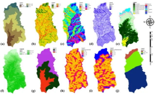
Fig. 3. Landslide conditioning factor used for landslide susceptibility mapping: (a) altitude, (b) slope, (c) aspect, (d) mean topographic wetness index, (e) landcover, (f) normalized difference vegetation index, (g) dominant soil,
(h) distance to river, (i) distance to lineaments and (j) rainfall
Index) methods were used to calculate the LSI (Landslide Susceptibility Index) for the study area. Both methods are bivariate statistical approaches which establishes relationship between the conditioning factors based on the distribution of the historical landslides (Guzzetti et al., 1999). FR method uses the landslide occurrence frequency for each class in each factor to provide the weightage whereas the SI uses the FR to derive the positive or negative information based on the log scale. Both methods have been widely used in in various studies (Yang et al., 2016; Zhang et al., 2016; Kayastha, 2015;
Regmi et al., 2014; Sarkar et al., 2013; Yalcin, 2008; Lee and Sambath, 2006). Suppose that j is a class within a factor i, then the FR is calculated as a ratio of density of landslide within a class of a factor to the density of landslide within the study area as follow:
(1)
where Ni, j is the number of the landslides in the class j within the factor i, Ai, j is the area of the class, NT is the total number of the landslides and AT is the total area of the study area. The LSI represents the relative susceptibility based on the historical information. The higher value indicates the frequency of landslide occurrence is high whereas lower value indicates low occurrence of landslide in the class area.
And the SI is calculated as log of the FR.
(2)
The positive value represents the high correlation whereas the negative is quite opposite i.e. low landslide density in the class of the factor. The overall landslide susceptibility (S) of each pixel is calculated after summation of all the LSIs as:
(3)
where LSIi is the FR or SI for the factor i, and n is the total number of the factors.
The performance of the results were measured based on the ROC (Receiver Operating Characteristics) analysis (Zhang et al., 2016). The method is widely used one that
measures how much the model was success in modeling and predicting the results. The value derived from ROC is AUC (Area Under the Curve) analysis which ranges from 0.5 to 1.
The value more than 0.5 is acceptable and value near to 1 is a good model (Swets, 1988).
3. Result and Validation
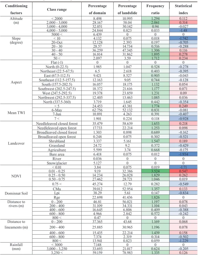
The correlation between the location of the landslides and the landslide conditioning factors prepared based on the Eq. 1 whereas the log of the FR provides the SI as shown in Table 1.
From Table 1, we can see that the class with lower NDVI i.e.
0.01 to 0.25 has higher relationship to landslide susceptibility in the range of 2000 to 3000 meters altitude. Similarly, higher slopes greater than 30 degree and areas with less TWI has shown higher information towards landslide occurrence. In contrast, if these area are at a distance more than 800 meters from lineaments showed negative information. The lower NDVI and bare area are the river floodplains which has very low slope, thus these classes has also negative information towards landslide occurrence.
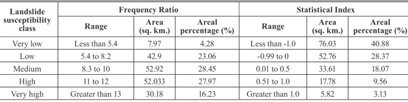
Based on Eq. 3, the landslide statistical index for both methods were derived, and thus landslide susceptibility maps were constructed. The range of the landslide susceptibility value for FR method were found to be 1.2 to 18 whereas for the SI were from -10.11 to 2.09. The higher vale are oblivious to have higher landslide susceptibility. The values were reclassified into five classes: very low, low, medium, high and very high as in the Table 2. For FR, classes were divided based on the natural breaks (jenks) as all the value were positive whereas the SI has negative values thus, only positive values were given high and very high class leaving rest low to medium susceptibility of landslide. In order to reduce the salt and pepper effect, the maps were smoothed using 8 cells majority filter. The final landslide susceptibility maps are shown in Fig. 4.
Visually, the maps were contrasting in the both low and high classes. In FR, the classes were evenly distributed in such way that all susceptibility class were visible equally in map, whereas in case of SI due to the negative index value, the very low and low classes were more in area. The class agreement in both methods were around 40% which
where is the number of the landslides in the class j within the factor i, is the area of the class, is the total number of the landslides and is the total area of the study area.
The LSI
where is the FR or SI for the factor i, and n is the total number of the factors.
where is the number of the landslides in the class j within the factor i, is the area of the class, is the total number of the landslides and is the total area of the study area.
The LSI
where is the FR or SI for the factor i, and n is the total number of the factors.
where is the number of the landslides in the class j within the factor i, is the area of the class, is the total number of the landslides and is the total area of the study area.
The LSI
where is the FR or SI for the factor i, and n is the total number of the factors.
Table 1. Spatial relationship between landslide and conditioning factors in the study area Conditioning
Class range Percentage Percentage Frequency Statistical
factors of domain of landslide ratio index
Altitude < 2000 8.498 10.995 1.294 0.112
(m) 2,000 - 3,000 28.167 58.04 2.061 0.314
3,000 - 4,000 32.051 30.142 0.94 -0.027
4,000 - 5,000 24.844 0.823 0.033 -1.48
5000 < 6.439 0 0 0
Slope < 10 4.132 0.075 0.018 -1.742
(degree) 20-Oct 12.128 2.393 0.197 -0.705
20 - 30 28.57 14.734 0.516 -0.288
30 - 40 36.259 47.345 1.306 0.116
40 - 50 16.814 31.862 1.895 0.278
50 < 2.097 3.59 1.712 0.234
Aspect
Flat (-1) 0 0 0 0
North (0-22.5) 1.985 1.047 0.528 -0.278
Northeast (22.5-67.5) 6.5 2.618 0.403 -0.395
East (67.5-112.5) 9.421 8.527 0.905 -0.043
Southeast (112.5-157.5) 12.163 9.05 0.744 -0.128
South (157.5-202.5) 16.057 18.175 1.132 0.054
Southwest (202.5-247.5) 18.372 21.616 1.177 0.071
West (247.5-292.5) 19.378 23.859 1.231 0.09
Northwest (292.5-337.5) 12.405 13.463 1.085 0.036
North (337.5-360) 3.719 1.645 0.442 -0.354
Mean TWI
< 5 24.453 43.381 1.774 0.249
6-May 62.756 52.132 0.831 -0.081
7-Jun 10.891 4.263 0.391 -0.407
7 < 1.901 0.224 0.118 -0.928
Landcover
Needleleaved closed forest 35.479 58.639 1.653 0.218
Needleleaved open forest 17.733 22.214 1.253 0.098
Broadleaved closed forest 1.303 0.898 0.689 -0.162
Broadleaved open forest 0.248 0.075 0.302 -0.521
Shrubland 3.337 5.161 1.547 0.189
Grassland 24.72 9.2 0.372 -0.429
Agriculture 5.599 3.74 0.668 -0.175
Bare area 6.418 0.075 0.012 -1.934
River 0.036 0 0 0
Snow/glacier 5.127 0 0 0
NDVI
< 0.01 3.84 0.075 0.019 -1.71
0.01 - 0.25 9.19 32.386 3.524 0.547
0.25 - 0.50 14.234 26.028 1.829 0.262
0.50 - 0.75 27.462 28.721 1.046 0.019
0.75 < 45.274 12.79 0.282 -0.549
Dominnat Soil CMu 39.012 52.954 1.357 0.133
Lpi 38.29 5.61 0.147 -0.834
Rge 22.698 41.436 1.826 0
Distance to 0 - 200 46.81 56.021 1.197 0.078
rivers (m) 200 - 400 31.109 34.331 1.104 0.043
400 - 600 16.645 6.806 0.409 -0.388
600 - 800 4.966 2.842 0.572 -0.242
800 < 0.47 0 0 0
Distance to 0 - 200 37.365 43.68 1.169 0.068
lineaments (m) 200 - 400 25.885 30.965 1.196 0.078
400 - 600 15.435 22.214 1.439 0.158
600 - 800 7.374 2.319 0.314 -0.502
800 < 13.941 0.823 0.059 -1.229
Rainfall < 3000 7.148 0 0 0
(mm) 3,000 - 3,250 33.693 21.017 0.624 -0.205
3,250 < 59.159 78.983 1.335 0.126
is mostly in low and high class falling in upper and lower region of the study area. The mid elevation range showed much disagreement due variation in FR and SI values. In terms of areas, FR showed around 30% and 45% of the study area to be low and high susceptible to landslides. And for SI, around 69% and 13% of the study area have low and high landslide susceptibility respectively. Overall the study areas having lower susceptibility to the landslide are mostly higher mountains covered in snow. The lower agricultural land along with the major settlement also have medium susceptibility.
The areas with higher susceptibility are mostly the non- settlement areas and frost, shrub lands in the steep hills.
In order to evaluate the accuracy of the derived susceptibly maps, ROC curve was used. Based on validation, training and whole dataset, ROC curves were produced and the AUC (Area Under Curve) for each case were calculated. As shown in Fig. 5, three ROC curves for each method were drawn. For
FR, the AUC value is 0.713 for validation, 0.725 for training and 0.722 for whole dataset. Similarly, for SI, the AUC value is 0.873 for validation, 0.886 for training and 0.883 for whole dataset. As the AUC value above 0.5 is considered as good result in ROC analysis, the values above 0.7 in this study shows reliable prediction using the both methods.
4. Conclusion
In this study, reliable landslide susceptibility maps were produced using two bivariate statistical models. The selected area was very remote area and lacked a reliable map for proper identification of landslide susceptible areas and mitigate the loss. The inventory was updated using Google Earth Pro images and ten conditioning factors were collected from various sources. Both FR and SI method, established a well relationship between the conditioning factors. Based on the derived LSIs, the study area was divided into five susceptible classes and showed mostly regions were less susceptible including the human settlements and agricultural lands. The high susceptible areas were mostly forest and steep hills in mid regions. Also, the AUC over 0.7 showed reliability of the result produced.
Fig. 4. Landslide susceptibility map produced by (a) Frequency Ratio and (b) Statistical Index
Fig. 5. ROC (Receiver Operating Characteristics) curves for the results from (a) FR and (b) SI
Table 2. Statistical index range and area of five landslide susceptibility classes Landslide
susceptibility class
Frequency Ratio Statistical Index
Range Area
(sq. km.) Areal
percentage (%) Range Area
(sq. km.) Areal percentage (%)
Very low Less than 5.4 7.97 4.28 Less than -1.0 76.03 40.88
Low 5.4 to 8.2 42.9 23.06 -0.99 to 0 52.76 28.37
Medium 8.3 to 10 52.92 28.45 0.01 to 0.5 33.61 18.07
High 11 to 12 52.033 27.97 0.51 to 1.0 17.78 9.56
Very high Greater than 13 30.18 16.23 Greater than 1.0 5.82 3.13
The study shows that successful application of the FR and SI methodologies can be a reliable source of information for landslide prone areas in hilly regions of Nepal. As, the study does not include the landslides followed after the inventory was made and the proximity effect as the area is small and the FR and SI can change for large or regional scale. This successful application of this study is next step for the preparation of regional scale map in whole district.
References
Acharya, T.D., Yang, I.T., and Lee, D.H. (2016), Geospatial technologies for landslide inventory: application and analy- sis to earthquake-triggered landslide of Sindhupalchowk, Nepal, Journal of the Korean Society for Geo-spatial Information Science, Vol. 24, No. 2, pp. 95-106.
Althuwaynee, O.F., Pradhan, B., Park, H., and Lee, J.H.
(2014), A novel ensemble bivariate statistical evidential belief function with knowledge-based analytical hierarchy process and multivariate statistical logistic regression for landslide susceptibility mapping, Catena, Vol. 114, No. 0, pp. 21-36.
Devkota, K., Regmi, A., Pourghasemi, H., Yoshida, K., Pradhan, B., Ryu, I., Dhital, M., and Althuwaynee, O.
(2013), Landslide susceptibility mapping using certainty factor, index of entropy and logistic regression models in GIS and their comparison at Mugling–Narayanghat road section in Nepal Himalaya, Natural Hazards, Vol. 65, No.
1, pp. 135-165.
Guzzetti, F., Carrara, A., Cardinali, M., and Reichenbach, P.
(1999), Landslide hazard evaluation: a review of current techniques and their application in a multi-scale study, Central Italy. Geomorphology, Vol. 31, No. 1–4, pp. 181- 216.
Kayastha, P. (2015), Landslide susceptibility mapping and factor effect analysis using frequency ratio in a catchment scale: a case study from Garuwa sub-basin, East Nepal, Arabian Journal of Geosciences, Vol. 8, No. 10, pp. 8601- 8613.
Lee, S. and Sambath, T. (2006), Landslide susceptibility mapping in the Damrei Romel area, Cambodia us- ing frequency ratio and logistic regression models,
Environmental Geology, Vol. 50, No. 6, pp. 847-855.
Petley, D., Hearn, G., Hart, A., Rosser, N., Dunning, S., Oven, K., and Mitchell, W. (2007), Trends in landslide occurrence in Nepal, Natural Hazards, Vol. 43, No. 1, pp.
23-44.
Pourghasemi, H., Pradhan, B., and Gokceoglu, C. (2012), Application of fuzzy logic and analytical hierarchy process (AHP) to landslide susceptibility mapping at Haraz watershed, Iran, Natural Hazards, Vol. 63, No. 2, pp. 965-996.
Regmi, A.D., Devkota, K.C., Yoshida, K., Pradhan, B., Pourghasemi, H., Kumamoto, T., and Akgun, A. (2014), Application of frequency ratio, statistical index, and weights-of-evidence models and their comparison in landslide susceptibility mapping in Central Nepal Himalaya, Arabian Journal of Geosciences, Vol. 7, No. 2, pp. 725-742.
Sarkar, S., Roy, A.K., and Martha, T.R. (2013), Landslide susceptibility assessment using information value method in parts of the Darjeeling Himalayas. Journal of the Geological Society of India, Vol. 82, No. 4, pp. 351-362.
Swets, J.A. (1988), Measuring the accuracy of diagnostic systems, Science, Vol. 240, No. 4857, pp. 1285-1293.
Uddin, K., Shrestha, H.L., Murthy, M.S.R., Bajracharya, B., Shrestha, B., Gilani, H., Pradhan, S., and Dangol, B.
(2015), Development of 2010 national land cover database for the Nepal, Journal of Environmental Management, Vol. 148, pp. 82-90.
van Westen, C.J., Castellanos, E., and Kuriakose, S.L.
(2008), Spatial data for landslide susceptibility, hazard, and vulnerability assessment: an overview, Engineering Geology, Vol. 102, No. 3–4, pp. 112-131.
Yalcin, A. (2008), GIS-based landslide susceptibility mapping using analytical hierarchy process and bivariate statistics in Ardesen (Turkey): comparisons of results and confirmations, Catena, Vol. 72, No. 1, pp. 1-12.
Yang, I.T., Acharya, T.D., and Lee, D.H. (2016), Landslide susceptibility mapping for 2015 earthquake region of Sindhupalchowk, Nepal using frequency ratio, Journal of the Korean Society of Surveying, Geodesy, Photogrammetry and Cartography, Vol. 34, No. 4, pp.
443-451.
Zhang, G., Cai, Y., Zheng, Z., Zhen, J., Liu, Y., and Huang, K.
(2016), Integration of the statistical index method and the analytic hierarchy process technique for the assessment of landslide susceptibility in Huizhou, China, Catena, Vol.
142, No. Supplement C, pp. 233-244.