1) Graduate student of Department of Construction & Disaster Prevention Engineering, Kyungpook National University, Korea 2) Department of Construction & Disaster Prevention Engineering, Kyungpook National University, Korea
Soil Erosion Modeling in the 3S Basin of the Mekong River Basin
Hoang Thu Thuy1)・ Giha Lee2)・ Wansik Yu†・ Yongchul Shin3) Received: April 5th, 2017; Revised: April 20th, 2017; Accepted: June 26th, 2017
ABSTRACT : The 3S Basin is described as an important contributor in terms of many aspects in the Mekong River Basin in Southeast Asia. However, the 3S Basin has been suffering adverse consequences of changing discharge and sediment, which are derived from farming, deforestation, hydropower dam construction, climate change, and soil erosion. Consequently, a large population and ecology system that live along the 3S Basin are seriously affected. Accordingly, the calculating and simulating discharge and sediment become ever more urgent. There are many methods to simulate discharge and sediment. However, most of them are designed only during a single rainfall event and they require many kinds of data. Therefore, this study applied a Catchment-scale Soil Erosion model (C-SEM) to simulate discharge and sediment in the 3S Basin. The simulated results were judged with others references’s data and the observed discharge of Strung Treng station, which is located in the mainstream and near the outlet of the 3S Basin. The results revealed that the 3S Basin distributes 31% of the Mekong River Basin’s total discharge. In addition, the simulated sediment results at the 3S Basin’s outlet also substantiated the importance of the 3S Basin to the Mekong River Basin. Furthermore, the results are also useful for the sustainable management practices in the 3S Basin, where the sediment data is unavailable.
Keywords : The 3S Basin, C-SEM model, Soil Erosion, The Mekong River Basin, Sediment Journal of the Korean Geo-Environmental Society
18(7): 21~35. (July, 2017) http://www.kges.or.kr
ISSN 1598-0820 DOI https://doi.org/10.14481/jkges.2017.18.7.21
1. Introduction
The Mekong River is measured as the largest river in Southeast Asia and ranked as the 21st largest river basin worldwide (MRC, 2011). Its transboundary covering a total area of 795,000 km2, which is dispensed among the six countries China, Myanmar, Thailand, Cambodia, Laos, and Vietnam (MRC, 2005). Additionally, it is also graded as the 12th longest river in the world (approximately 4,909 km) and the 8th largest water discharge (the mean discharge equals 15,000 m3/s) (MRC, 2003). Three of the biggest discharge and sedimentation contributors into the Mekong River’s mainstream are Srepok, Sesan, and Sekong Rivers, which are known informally as “3S” rivers (Kondolf et al., 2014). For example, the 3S Basin’s annual sediment load is calculated at 10-25 Mt/year or 10-20% of the Mekong River Basin’s total sediment (Watt, 2015). Moreover, the 3S Baisn also offers a diversity of fishes and supports food production and working opportunities for communities through the migration of fish plus water flow and sediment. It is characterized by 329 fish species, which is estimated to be equal to 42% of the 781 fish species
occurring in the Mekong River Basin (Baran et al., 2013).
Besides, Piman et al. (2012) stated that the 3S Basin is also a home of over 2.5 million people. Therefore, much attention has been concentrated on the 3S Basin, particularly, calculating and controlling soil erosion as well as water quality are considered as cases of emergency.
In recent, many factors have been causing the alteration in discharge and sediment concentration of the 3S Basin such as land use, water demand, hydropower dams, and climate change. According to statistics, the 3S Basin, especially in Vietnam and Laos, has been undergoing rapid hydropower development due to economic growth and electricity demand (Piman et al., 2012). There is an entirety of 45 dams proposed in the 3S Basin, in which 22 dams belong to the Sekong, 13 dams are located on the Sesan, and 10 dams are placed on the Srepok (ADB-RETA, 2010a). The operation of existing hydropower dams is a great source of economic benefits.
Nevertheless, it has caused severe negative impacts such as poor water quality, soil erosion, deposition problem, a decrease of fish habitat and species, the damage of sustenance, and economic guarantee (Groner, 2006). Furthermore, continued
deforestation combined with the development of hydropower dam led to soil erosion on steep slopes and an increase in the frequency of flash floods (Watt, 2015).
The amount of sediment keeps an important role in the great biological and ecological diversity of the 3S Basin.
However, in the United States Agency for International Development (Wild and Loucks, 2014) document researching about assessment of the potential for controlling the amount of sediment and evaluating its influences on energy manufacture in the 3S Basin, it is remarked that in the Definite Future Scenario, about 44-59% (or equals around 10-13.3 Mt/year) of the 3S Basin’s sediment load will be trapped in reservoirs.
And in the Foreseeable Future Scenario (2030), the sediment trapping will fluctuate from 72% to 78% (around 16.2-17.7 Mt/year) (Wild and Loucks, 2014). In another research study, it is calculated that the discharged sediment load from the 3S Basin will be reduced to 1.6 Mt/year (USAID, 2014).
It is easy to realize that the 3S Basin is a vulnerable area because of soil erosion. Given the current issue and problems with the soil erosion in the 3S Basin, a proper evaluation deal with soil erosion should be considered carefully, in order to provide the essential and important information for countermeasures (structural or nonstructural) against the soil erosion problem. The study consists of two specific objectives:
simulating the rainfall-runoff-sediment for the 3S Basin and discovering how important the 3S Basin was to the Mekong River Basin in terms of discharge and sediment concentration.
The purpose of this study is to analyze how much soil erosion occurs in the 3S basin by using the developed soil erosion model and to use it as basic data for establishing a soil erosion management.
Choosing an appropriate model is one of the most signi- ficant steps to get desired results in studies and projects.
Selecting the suitable model is based on different aspects of specific researches, project requirements, characteristics of considered catchments, and many other factors. In general, basing on input and output relationship the models used for prediction and assessment of soil erosion can be categorized into three main types: empirical, conceptual, and physically- based models. In general, estimating soil loss need various information relating to rainfall, soil type, land cover, topo- graphy, rainfall, and climate. Therefore, it is essential to develop and apply a physically-based distributed rainfall- sediment-runoff model (Apip et al., 2008). There are some
popular distributed sediment runoff models which are designed to estimate sediment runoff during the particular rainfall event such as ANSWERS, WEPP, and LISEM. However, the disadvantages of most of them are that the models require comprehensive spatially and temporally variable data input for sizeable catchment and long-term simulations (Merritt et al., 2003; Apip et al., 2008). Besides, study areas have often unavailable data and heterogeneous soil erosion pattern, especially the 3S Basin. As a result, to simulate the sediment in the 3S Basin, the spatially distributed hydrologic model of rainfall-runoff-sediment yield simulation, C-SEM (Catchment scale soil erosion model), was applied to three sub-basins (SeamPang, VoeunSai, and Lumphat Basins) in the 3S Basin and the outlet of the 3S Basin for two years (2005-2006).
This article has been organized in the following way. After the introduction, section 2 introduces a rainfall-runoff-sediment yield model, which was applied into target basins. Section 3 introduces a study area, used data, model setup, and calibration.
Section 4 presents the model application results by comparing the observed discharge and sediment with simulated results, and addresses the results of percentages of simulated yearly discharge and sediment of each station (Lumphat, VoeunSai, SeamPang) and the outlet of the 3S Basin. Finally, the major conclusions are summarized in section 5.
2. Catchment scale soil erosion model (C-SEM)
To demonstrate transportation capacity of surface flow, this study used an operative spatially distributed erosion model which comprised two basic element models (Govers, 1990; Apip, 2008). The first method is a rainfall-runoff module which is grounded on the kinematic wave method for subsurface and surface flow with a conceptual relation- ship between stage and discharge (Tachikawa et al., 2004;
Lee et al., 2013). The second method is an erosion-sediment yield module which is constructed on the unit stream power method of Yang (1972) (Lee et al., 2013). Each of the models is explained in more detail as follows.
2.1 Rainfall-runoff module
Rainfall-runoff process expresses how water flow occurs on and below a ground surface and a movement of flow
Fig. 1. Schematic sketch of a catchment modeling using DEM (Tachikawa, 2011)
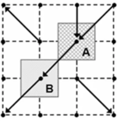
Fig. 2. Schematic sketch of the KWMSS slope elements for defining the drainage network (Lee et al., 2013)
Fig. 3. Relationship between stage and discharge of the KWMSS (Lee, 2008)
water (Shiiba et al., 2008). Therefore, to simulate soil erosion, a rainfall-runoff module must precisely visualize the spreading of rainfall, infiltration into the ground, and rainfall runoff routing from the channel sections to an outlet of the catchment (Julien et al., 1995). This study applied the cell-based one- dimensional kinematic wave method for subsurface-surface flow simulation (KWMSS), which was first presented by Takasao and Shiiba (1988) and extended by Tachikawa et al.
(2004). The model can realize both saturated and unsaturated flow mechanisms, which is suitable for the long-term runoff simulation from dry to humid seasons continuously (Tachikawa, 2011).
In this method, the drainage network, which is interpreted by hillslope and channel elements from the flow direction map extracted from DEM, determines a rainfall runoff direction (Shiiba et al., 1999). Therefore, to express each hillslope and channel elements, the DEM is divided into an orthogonal matrix of the squares which are formed by nodes and being considered as sub-basins or grid cells (Chaffe et al., 2014) (Figure 1). Figure 2 represents a schematic topographic description of KWMSS. The hydrology variables such as
water flux are indicated by the direction of the arrows. The rainfall over all hillslope elements, flows one-dimensionally into the river nodes and routes to the catchment outlet (Lee et al., 2013).
In the rainfall-runoff transformation which is conducted by KWMSS, it is assumed that a permeable soil layer covers all hillslope elements (Lee et al., 2013). Furthermore, the kinematic wave also presumes that rainfall intensity is always smaller than the infiltration rate capacity. Therefore, rainfall is assumed that it is straight inserted to subsurface or surface flow depending on the depth of the area where rainfall dropped without considering the initial rainfall losses due to vertical water flow such as infiltration effects (Chaffe et al., 2014). Moreover, it is also assumed that the kinematic wave appears as constant, unsteady flow, the water surface and bed are parallel, and the hydraulic gradient is equivalent to the slope (Chaffe et al., 2014). Figure 3 displays the relationship between stage and discharge in KWMSS.
Basing on the condition and state of soil and rainfall, the flow mechanism is divided into three types: (1) subsurface flow goes through capillary pores (unsaturated flow); (2) subsurface flow goes through non-capillary pore (saturated flow); and (3) surface flows on the soil layer with uniform thickness (overland flow) (Owens and Collins, 2006). When the equivalent water depth is higher than the water depth ( ≤ ≤ ), the flow is estimated by Darcy law with an unsaturated hydraulic conductivity and velocity . If the depth of water surpasses the equivalent depth for the un- saturated flow (≤ ≤ ), the soil is termed saturated (Lane et al., 1988). The saturated subsurface flow is calculated by Darcy law by using saturated hydraulic conductivity and the average velocity in the downslope direction is (Tachikawa, 2011; Apip et al., 2012). The surface flow occurs and is calculated by the Manning’s equation if the water depth is
Fig. 4. Erosion and deposition process of C-SEM at hillslope elements (Kim et al., 2015)
higher than the soil layer D (Tachikawa, 2011). The discharge with unit width (q) in unsaturated, saturated soil, and surface flow cases are calculated by the approximation corresponding to stage-discharge relationship (Equation 1) and the continuity equation (Equation 2) (Tachikawa et al., 2004).
≤ ≤
≤ ≤
≤
(1)
rxt (2)
where h (m) is water depth; q (m2/s) is the flow rate of discharge hillslope element, r is effective rainfall intensity,
(m/s), (m/s), (m/s),
(m1/3/s); , is the slope gradient, (m/s) is the hydraulic conductivity of the capillary soil layer, (m/s) is the hydraulic conductivity of the non-capillary soil layer, n (m-1/3s) is the roughness coefficient, ds (m) is the water depth matching to the water content, and dc (m) is the water depth according to maximum water content in the capillary pore (Lee et al., 2013). The values of water , , and
are optimized if needed.
2.2 Erosion-sediment yield module
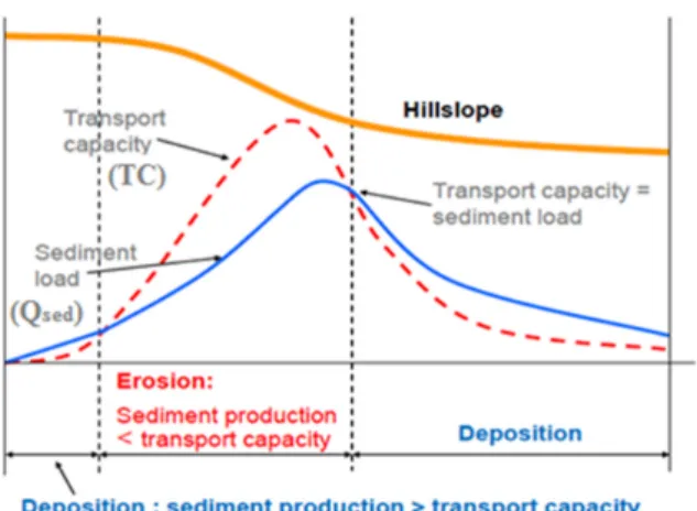
The algorithm of the erosion-sediment yield module is subject to the unit stream power notion and dependent on the relationship between transport capacity (TC) and sediment supply (Qsed) (Lee et al, 2013). As shown in Figure 4 both erosion and deposition can be determined by comparing the
value of TC to Qsed. When the surface runoff happens in a grid cell and the TC of the flow is larger than (Qsed) from the upper grid cell, the sediment of TC-Qsed will be yielded or erosion happens (Apip, 2008). On the other hand, if Qsed
is bigger than TC, the sediment of Qsed -TC will be built up in a grid cell or deposition happens (Sayama, 2003; Apip, 2008; Lee et al, 2013). The theory of the unit stream power is used to estimate the transportation capacity of overland flow which determines the rate of sediment yield or deposition in each grid-cell (Apip, 2008).
The sediment transport procedure contains various sediment transport sources, including soil detachment by raindrop (DR) and hydraulic detachment or deposition moved by overland flow (DF) (Apip et al., 2008). The model is subject to the essential assumption, which states that the sediment is yielded when overland flow happens and the eroded sediment is transported by overland flow to the river channel (Apip et al., 2008). To calculate erosion-sediment yield, the continuity equation representing DR and DF was adopted (Apip, 2008).
(3)
(4)
where C is the sediment concentration in the overland flow (kg/m3); hs is the depth of overland flow (m); qs is the discharge of overland flow (m3/s); e is the net erosion (kg/m2/hr); DR (rainfall detachment); and DF (flow detachment).
The DR is given by using an empirical equation with a supposition that the soil detachment rate is proportional to the kinetic energy of effective rainfall and decreases with increasing overland flow depth (hs) (Apip, 2008) (Equation 5). The DF is calculated as a function of surface flow and transport capacity (TC), which is described as the maximum value of sediment concentration to transport for each grid-cell (Anderson and Burt, 1985) (Equation 6).
(5)
(6)where k (kg/J) is the soil detachability, KE (J/m2) is the total kinetic energy of the net rainfall, b is the exponent to be
Fig. 5. Position of the 3S Basin (Sekong, Sesan, and Sprepok Basins)
tuned, and α is the non-dimensional detachment/deposition efficiency factor.
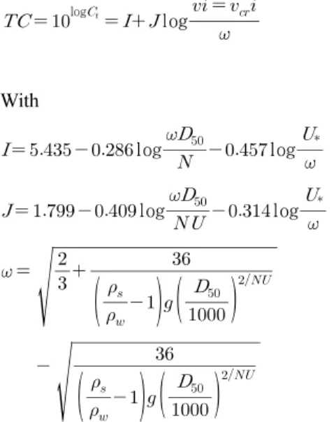
The sediment transportation capacity (TC) is calculated based on the Unit Stream Power (USP) theory which can be used for sediment transport in the open channels and surface land erosion (Yang, 1973). Yang (1973) also declared that the value of the TC rested on the particle settling velocity, shear velocity, grain size, kinematic viscosity of the water, and water density (Equation 7).
log log
(7)
With
log
log
log
log
where (mg/l) is the total sediment concentration, (m/s) is the unit stream power ( is the surface flow velocity in m/s and is the slope gradient m/m), (m/s) is the critical unit stream power ( is the critical flow velocity), (m/s) is the sediment fall velocity calculated by Rubey’s equation,
is the sediment particle density (kg/m3), is the water density (kg/m3), is the specific gravity (m/s2); is the median of grain size (mm), is the kinematic viscosity of the water (m/s2), and (m/s) is the average shear velocity.
3. Model application
3.1 Study area and data
The Sesan, Srepok and Sekong basins (3S Basin) (Figure 5) are located in the east of the Mekong’s mainstream with a whole area of 78,650 km2, of which the Sekong is in the north with 28,820 km2 area, the Sesan covering 18,890 km2
area is in the center, and the Srepok located in the south has the largest area with 30,940 km2 (IUCN, 2015). The total area of the 3S Basin is shared by three countries: Cambodia (33%), Laos (29%), and Vietnam (38%) (Piman et al., 2012).
The Central Highland of Vietnam, a source of three rivers, is a place where the Sekong flows through the Laos before joining with the Sesan and Srepok Rivers over the distance of about 40 km before creating a confluence with the Mekong River at Strung Treng station (ADB-RETA, 2010a). Contributing around 17-20% of the total Mekong mainstream’s annual flow, which means 91,000×106 m3 or an average of 2,886 m3/s, and about 10% of the total Mekong River’s sediment, the 3S Basin is evaluated as the largest tributary contribution as well as a significantly important area to the Mekong River Basin (Adamson et al., 2009; ADB-RETA, 2010a).
Geophysically, the elevation of the 3S Basin changes from mountainous areas in the east to plains in the west and ranges from 50 m to 2,409 m above sea level at the concourse with the Mekong River at Strung Treng station (IUCN, 2015).
Therefore, the Sesan basin has the highest average elevation, at 558 m, followed by the Sekong basin at 576 m and the Srepok basin at 399 m (IUCN, 2015). Not only seasonal monsoon but also topography has strong influences on annual
Table 1. Locations of Strung Treng station, outlet of the 3S Basin, the discharge and sediment concentration stations in the 3S Basin
Station Longitude (degree) Latitude (degree)
SeamPang 106.389642 14.114826
VeounSai 106.884834 13.968580
Lumphat 106.975629 13.496744
Outlet of the 3S Basin 105.995606 13.545988
Strung Treng 105.933548 13.522047
Fig. 6. Position of discharge and sediment stations and outlet of the 3S Basin
Fig. 7. The calibration and validation process of C-SEM methodology rainfall precipitation (varying from 1,100 mm/year to 3,800
mm/year) and average annual temperature (ranging from 22oC to 27oC) (Piman et al., 2012; Shrestha et al., 2016). Having higher elevation, the upper Sekong basin has more precipi- tation and slightly cooler average temperatures than Sesan and Srepok Basins. The International Union for Conservation of Nature (IUCN, 2015) stated that along the border between Laos and Vietnam, the average annual precipitation can exceed 2,800 mm/year.
3.2 Model setup and calibration
This research used five main types of data sources: DEM, landcover, rainfall, discharge, and sediment. The DEM was derived from HydroSHED for Asia with 1 km × 1 km spatial resolution. Then, the DEM was put in Arc GIS to calculate the flow direction and flow accumulation. The landcover map was taken the USGS Land Cover Institute is 0.5 km MODIS–based Global Land Cover Climatology (in ten years:
2001-2010), which contains 17 different types. The rainfall data is taken from the Asian Precipitation Highly Resolved Obser- vational Data Integration towards Evaluation (APHRODITE) of Water Resource (conducted by the Research Institute for Humanity and Nature (RIHN) and the Meteorological Research Institute of Japan Meteorological Agency (MRI/JMR)). The APHRODITE rainfall data is a daily gridded precipitation, which covers a 57 year time period (from 1951 to 2007).
The observed discharge data was taken from the discharge hydrograph on the MRC website. The observed sediment was collected by researchers. Both discharge and sediment data are daily and discontinuous. However, the rainfall-sediment- runoff model requires the hourly data. As a result, the daily APHRODITE rainfall and observed data were divided by 24, which reduced the accuracy of the model. Table 1 and Figure 6 show the positions of sediment and discharge stations
in the 3S Basin and the outlet of the 3S Basin.
The hydrological data set in the period from 1st June 2005 to 30th November 2005 at VeounSai station was selected as an example for the calibrating discharge. However, the only Lumphat station has observed sediment concentration. Therefore, after applying the optimized discharge parameters which were taken from calibrating parameter at VeounSai station, the sediment concentration parameters at Lumphat station were calibrated in the same period. Then, optimized discharge and sediment concentration parameters were applied in all stations and the outlet of the 3S Basin in a two year period (2005-
Table 2. Roughness coefficient for specific types of land use (Vieux, 2004)
No Land use / land cover classification Manning’s n
1 Water area 0.030
2 Urbanization 0.015
3 Eroded land 0.035
4 Marsh 0.050
5 Grassland 0.130
6 Forest 0.100
7 Paddy field 0.050
8 Cropland 0.035
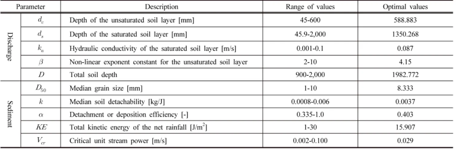
Table 3. Practicable parameter range of model calibration and optimum parameter values
Parameter Description Range of values Optimal values
Discharge
Depth of the unsaturated soil layer [mm] 45-600 588.883
Depth of the saturated soil layer [mm] 45.9-2,000 1350.268
Hydraulic conductivity of the saturated soil layer [m/s] 0.001-0.1 0.087
Non-linear exponent constant for the unsaturated soil layer 2-10 4.15
Total soil depth 900-2,000 1982.772
Sediment
Median grain size [mm] 1-10 8.333
Median soil detachability [kg/J] 0.0008-0.006 0.0037
Detachment or deposition efficiency [-] 0.335-1.0 0.403
Total kinetic energy of the net rainfall [J/m2] 1-30 15.907
Critical unit stream power [m/s] 0.002-0.100 0.029
2006). The process of calibration and validation is shown in Figure 7.
While the Thiessen Polygon method was chosen to calculate the rainfall dissemination, the subsurface and surface flow was calculated by Equations 1 and 2. The calibration and validation models were executed at 1 hour-step for the hydrological data set.
In the erosion-sediment yield module used the Manning’s roughness coefficient. It is affected directly by land cover and plays an imperative role in simulating the surface flow and soil detachment (Lee et al., 2013). Due to lack of the detailed Manning’s roughness coefficient information of land cover for the whole 3S Basin, the land cover was reclassified from 17 types as being mentioned before into 8 types and one unique value for river channel (0.005). The values of Manning’s roughness coefficient are given by the water controlling information system (WAMIS; http://www.wamis.go.kr), based on (Vieux, 2004), as summarized in Table 2.
The SCE-UA model (Duan et al., 1994) only provides one hydrologic output variable while the C-SEM model contains two modules: a rainfall-runoff and an erosion-sediment yield
module. It means that the C-SEM was used twice. The first process is to offer the output variable-discharge and optimal parameter values related to discharge by using the objective function: root mean square error (RMSE) of stream flow (Equation 8):
(8)where is the observed stream flow at time ,
is the simulated stream flow at time , using the compromise solution parameter set , and is the number of available data.
Similarly, the second process is the output variable˗sediment and optimal parameter values related to sediment (Table 3) by using the objective function: Root mean square error (RMSE) of sediment discharge (Equation 9):
(9)The practicable parameter ranges were established based on reference published by (Apip, 2008; Lee et al., 2013).
The calibrated parameter values of the model are stated in the last column of Table 3.
It is difficult to have a station which has the observed sediment and discharge at the same period. Therefore, after getting the optimal parameter from calibrations at VeounSai and Lumphat stations, it was supposed that process parameters and some physical parameters in Table 3 are spatially homo- geneous over the study catchment and were then applied for Lumphat, SeamPang, VoeunSai stations, and the outlet of
Fig. 8. Comparison of observed discharge with simulated discharge at VeounSai station for the period 1st June - 30th November 2005
Fig. 9. Comparison of observed sediment concentration with simulated concentration at Lumphat station for the period 1st June - 30th November 2005
the 3S Basin during the time period from 1st January 2005 to 31st December 2006. The Nash-Sutcliffe efficiency (NSE) was used to evaluate model applicability (Equation 10):
∑
∑
(10)
where is the th observation for the constituent being evaluated, is the th simulated value for the constituent being evaluated, is the mean of observed data for the constituent being evaluated, and is the total number of observations.
4. Application Results
We applied the calibrated model to rainfall-runoff-sediment yield simulation by using the VeounSai station’s observed discharge data and observed sediment concentration data at Lumphat station for six months (from 1st June to 30th November 2005). Figure 8 illustrates the observed data versus simulated discharge results at VeounSai station. And Figure 9 shows the comparison between observed data versus simulated sediment concentration results at Lumphat station in the 1st June to 30th November 2005 time period.
Although the simulated parameters are not really close to
Fig. 10. Comparison of simulated discharge with observed discharge at VoeunSai station for the period 2005-2006
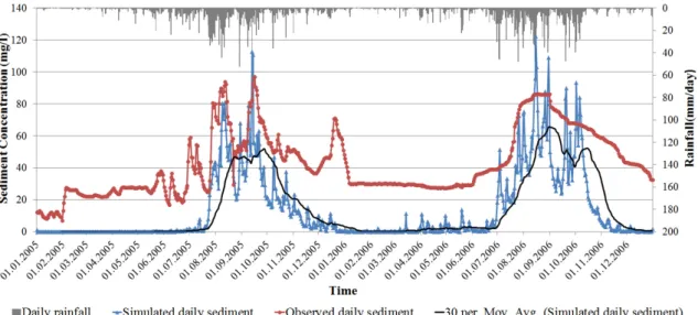
Fig. 11. Comparison of simulated sediment concentration with the observed sediment concentration at Lumphat station for the period 2005-2006
Table 4. Model performances in model phase in VoeunSai and Lumphat stations for the period 2005-2006
Observed-simulated discharge at VeounSai station
Observed-simulated sediment concentration at Lumphat station
NSE 0.67 -1.52
RMSE 526.56 31.97
the observed data because of many reasons, the model was generally successful in symbolizing broad trends in water discharge in VeouSai station. However, the result of simulating sediment concentration in the river water was not as precise as the case of hydrologic simulate at Lumphat station.
After calibrating stage, optimized parameters were used to validate discharge and sediment concentration at the outlet of the 3S Basin and all stations in the 3S Basin (VoeunSai, SeamPang, and Lumphat Stations) for two years (2005-2006).
Figures 10 and 11 express the simulated discharge results at VeounSai station and sediment concentration results at Lumphat station for the period from 2005 to 2006, basing on the optimized parameters.
The Nash-Sutcliffe efficiency (NSE) was calculated to assess the model applicability. At the VeounSai station, the NSE
and RMSE values between observed discharge and simulated discharge are 0.67 and 526.56, respectively. It signified that the simulated results are generally successful for VoeunSai station. However, the NSE value is only -1.52 and the RMSE value is 31.97 for the simulated and observed sediment concentration at Lumphat station (Table 4).
There is very little observed sedimentation data available in the Mekong River Basin, especially the 3S Basin. Specifically,
(a) (b)
Fig. 12. (a) Value and (b) percentage of simulated yearly mass discharge of each station in the 3S Basin in 2005
(a) (b)
Fig. 13. (a) Value and (b) percentage of simulated yearly mass discharge of each station in the 3S Basin in 2006 this study used data from two main sources; the Mekong
River Commission (MRC) website and researchers. Observed data was available at two stations (Lumphat and VeounSai).
At Lumphat station, observed water level data (2000-2005) and observed discharge data (2000-2004) were taken from the graphs on the MRC website. The researchers only provided observed water level data (2000-2014) and discontinuous daily sedimentation data (2005-2006). However, the C-SEM modeling needed continuous and hourly data to calibrate and validate parameters. Therefore, the trend lines showing water level–discharge and discharge–sedimentation relationships were used to interpolate and extrapolate continuous daily sedimen- tation data in the period from 2005 to 2006. Then, the daily observed data was divided into 24 to get hourly data. Because of these procedure modifications, the observed sediment data was modified. It made the NSE value of observed and simulated sedimentation at Lumphat station low (NSE = -1.57).
As a result, the validated sediment concentration results could not fit well with the observed data in a two year period (2005-2006) even thought they were calculated by using
optimized parameters.
At the VeounSai station, the observed sedimentation data is unavailable. The observed daily discharge and water level data were taken from graphs on the MRC website. However, the time period within which data is available is restricted to only two years (2000-2001), while the researchers only supplied observed water level data from 2000 to 2014. In addition, the observed data on the MRC website and from researchers are slightly different. Consequently, to get the observed daily discharge data in the period 2005-2006, it was necessary to find the trend line and equation showing the relationship between water level-discharge data from the two data sources. Similar to the Lumphat station, the observed daily data was divided into 24 to get hourly data for calibration and validation processes. Therefore, the NSE value of observed and simulated discharge at VeounSai station can be greater than the present value (NSE = 0.67) if the observed discharge data is taken from only one data source and the observed hourly discharge data is obtainable.
The value and percentage of simulated yearly discharge
(a) (b)
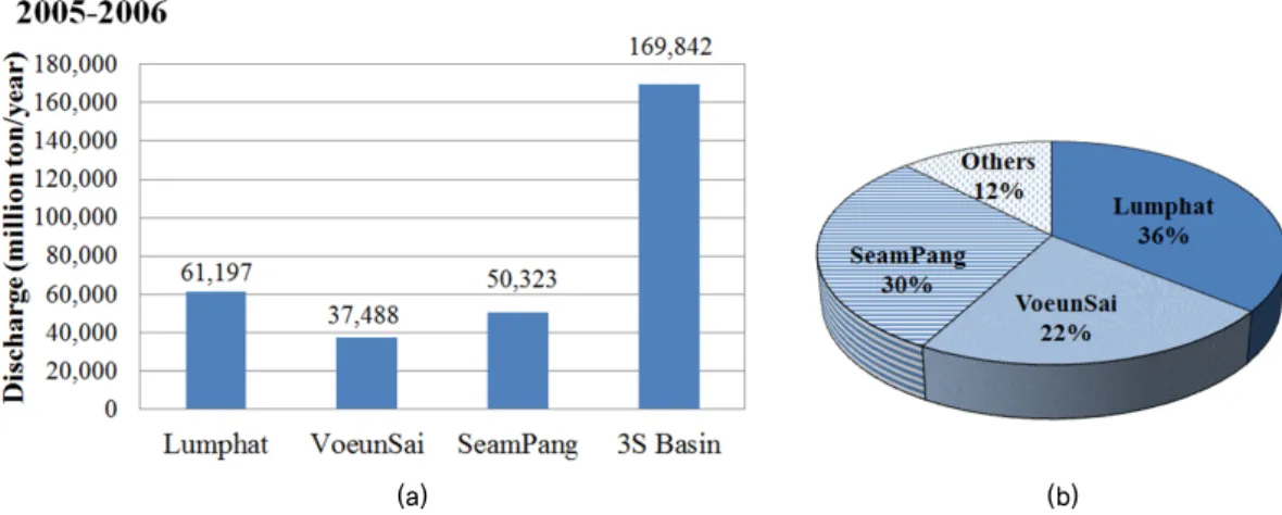
Fig. 14. (a) Value and (b) percentage of simulated average yearly mass discharge of each station in the 3S Basin in the period 2005-2006
Fig. 15. Simulated yearly sediment of each station in the 3S Basin in 2005
Fig. 16. Simulated yearly sediment of each station in the 3S Basin in 2006
Fig. 17. Simulated average yearly sediment of each station in the 3S Basin in the period 2005-2006
of each station (Lumphat, VoeunSai, SeamPang Stations) and the outlet of 3S Basin in 2005 and 2006 are shown in Figures 12, 13 and the average value is shown in Figure 14.
All these figures indicate that Lumphat station contributed the largest runoff volume to the total discharge of the 3S Basin, the second one is SeamPang station, followed by VoeunSai station in the third position. The percentage of simulated average yearly discharge of each station in the 3S Basin for the period 2005-2006 are 36% (61,197 Mt/year) in Lumphat station, 30% (50,323 Mt/year) in SeamPang station, 22% (37,488 Mt/year) in VoeunSai station and 12% in the rest of the 3S Basin. It is obvious to recognize that the total discharge of three stations (Lumphat, VoeunSai, and SeamPang Stations) is not equal to the discharge at the outlet of the 3S Basin. One of the reasons is that the total area of sub-basins having outlets as the above three stations is smaller than the area of the 3S Basin (Figure 6).
In contrast, although the VeounSai station has the least discharge, it has the largest sediment concentration with 47 mg/l (2005) and 51 mg/l (2006), followed by SeamPang station with 29 mg/l (2005) and 27 mg/l (2006) sediment concentration.
Lumphat station is ranked in the third position with the least amount of sediment concentration (12 mg/l (2005) and 16 mg/l (2006)) though it has the largest discharge among stations (Figures 15, 16). As a result, the amount of simulated average yearly sediment concentration for the period 2005- 2006 of VoeunSai, SeamPang, Lumphat Stations are 49 mg/l;
28 mg/l; and 14 mg/l respectively (Figure 17). Additionally, the total sediment contribution of the 3S Basin is not equal to the sediment at the outlet of the 3S Basin because the sediment transportation process is composed of both erosion
(a) (b)
Fig. 18. (a) Value and (b) percentage of simulated average discharge of the 3S Basin in the period 2005-2006 with the observed average yearly discharge of Strung Treng station in the period 2000-2001
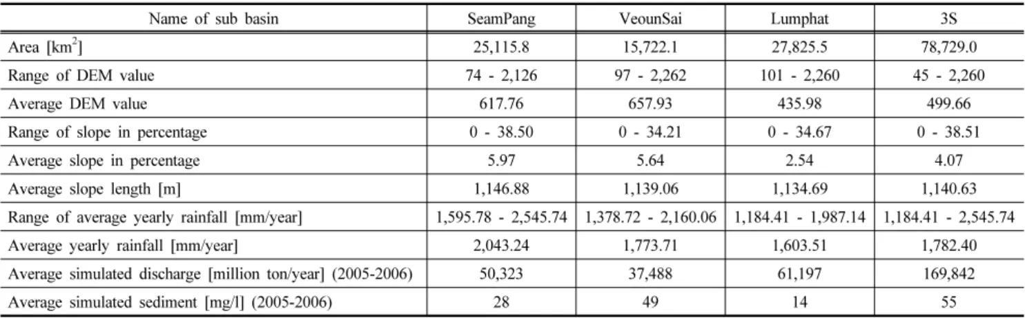
Table 5. Comparison of C-SEM results among sub-basins in the 3S Basin
Name of sub basin SeamPang VeounSai Lumphat 3S
Area [km2] 25,115.8 15,722.1 27,825.5 78,729.0
Range of DEM value 74 - 2,126 97 - 2,262 101 - 2,260 45 - 2,260
Average DEM value 617.76 657.93 435.98 499.66
Range of slope in percentage 0 - 38.50 0 - 34.21 0 - 34.67 0 - 38.51
Average slope in percentage 5.97 5.64 2.54 4.07
Average slope length [m] 1,146.88 1,139.06 1,134.69 1,140.63
Range of average yearly rainfall [mm/year] 1,595.78 - 2,545.74 1,378.72 - 2,160.06 1,184.41 - 1,987.14 1,184.41 - 2,545.74
Average yearly rainfall [mm/year] 2,043.24 1,773.71 1,603.51 1,782.40
Average simulated discharge [million ton/year] (2005-2006) 50,323 37,488 61,197 169,842
Average simulated sediment [mg/l] (2005-2006) 28 49 14 55
and deposition. Therefore, part of the sediment is trapped on the way and cannot be drained into the outlet of the 3S Basin.
Table 5 summarized the C-SEM results among sub-basins in the 3S Basin. It is easy to realize that the Lumphat sub- basin has the biggest area (27,825.5 km2), which nearly doubles VeounSai sub-basin. Consequently, although the average yearly rainfall of this sub-basin is smallest (1,603.51 mm/year), the average simulated discharge (2005-2006) is higher than the rest of sub-basins in the 3S Basin with 61,197 Mt/year.
Nevertheless, the flat topography with the slightest average slope in percentage (2.54%) and smallest average DEM value (435.98) is one of the reasons making the amount of soil deposition much more than the amount of soil erosion.
Therefore, the average simulated sediment (2005-2006) of Lumphat station (14 mg/l) is less than sediment concentration at SeamPang station (28 mg/l) and VeounSai station (49 mg/l).
Comparing with VeounSai sub-basin, SeamPang sub-basin has higher average slope in percentage (5.97%), average slope length (1,146.88 m), and average yearly rainfall (2,043.24
mm/year). However, the average DEM value of the VeounSai sub-basin (657.93) is bigger than SeamPang’s one (617.76).
Beside the different land cover management factor, the average DEM value is also an important fact contributing to the larger average simulated sediment (49 mg/l) of the VeounSai sub- basin compared to SeamPang sub-basin (28 mg/l).
Normally, the simulated results should be compared to the observed data at the same station to assess an accuracy of the model. However, there are no observed discharge and sediment concentration data of the outlet of the 3S Basin.
Therefore, the observed data at Strung Treng station, which belongs to the mainstream was opted for to be compared with the simulated results in the outlet of the 3S Basin.
Nevertheless, Strung Treng station has only observed discharge data for the period between 2000 and 2001 and it does not have observed sediment concentration data. As a result, the observed average yearly discharge of Strung Treng station for the period 2000-2001 was calculated to compare with the simulated average yearly discharge of the 3S Basin (2005-2006). Figure 18 shows that the 3S Basin contributes
Fig. 19. Sediment concentration mass at the outlet of the 3S Basin in 2005 and 2006
31% (169,842 Mt/year) of the main stream’s discharge.
Comparing with other references, this figure is higher. For example, Adamson et al. (2009) and ADB-RESTA (2010a) stated that the annual flow of the 3S Basin is 91,000×106 m3 or 2,889 m3/s (around 17-20% annual discharge of the Mekong river’s main stream). However, the study’s results can be accepted because the time period comparison is short and different. While the simulated average yearly discharge of the 3S Basin was calculated in the period 2005-2006, the period time to calculate the observed average yearly discharge of Strung Treng station was from 2000 to 2001. Generally, the results confirmed again the magnitude of the 3S Basin to the Mekong River Basin into contributing discharge and sediment concentration.
After calculating the average yearly discharge and sediment concentration in the outlet of the 3S Basin, the sediment concentration mass was calculated to compare with the results from previous references. The settled sediment mass depends on its bulk density (Wild and Loucks, 2014). Basing on the a survey of reservoir sedimentation at various locations in the United Stated which were performed by Lara and Pemberton (1963), it is supposed that the value of sediment concentration bulk density is 1,200 kg/m3. Therefore, the sedimentation mass was estimated by below formula:
× (11)
where: m: mass (kg), V: volume (m3), D: bulk density (kg/m3).
The sediment concentration mass values at the outlet of the 3S Basin is 10 Mt/year (2005) and 13 Mt/year (2006) (see Figure 19), and the average value is 11.5 Mt/year. In other references, Watt (2015) remarked that annual sediment
load of the 3S Basin is 10-25 Mt/year (or 10-20% annual sediment load of the Mekong River’s). Therefore, this result is acceptable.
5. Summary and Conclusion
Basing on the results of average annual soil loss, the 3S Basin was analyzed more deeply by using the C-SEM modeling. The model simulated rainfall-runoff-sediment for the 3S Basin, and justified the importance of the 3S Basin to the Mekong River Basin in terms of discharge as well as sediment concentration. The surface runoff and soil erosion simulation models are evaluated as valuable models to accurately provide the essential and important information such as discharge and sediment yields not only in monitoring sites but also in ungauged catchments (Lee et al., 2013).
Nevertheless, although this study applied one kind of these models, it was found that the simulated results were not well distributed comparing with the observed data because of several difficulties. The first is that not all types of data were available. For example, the C-SEM modeling requires hourly discharge and sediment data. However, the only provided available observed data was not only daily, but also discontinuous. The second difficulty was data uncertainty and lastly, the time period comparison is short and different between the simulated results and the observed data. In addition, there was no observed sediment concentration in Strung Treng station to compare with the simulated sediment result in the outlet of the 3S Basin. However, the simulated result showed the importance of the 3S Basin to the Mekong River Basin in terms of discharge and sediment. Specifically, it indicated the amounts and percentages of discharge and sediment concentration of each station in the 3S Basin com- paring to the whole 3S Basin. In addition, it also demonstrated that the 3S Basin contributed a large percentage of the discharge and sediment in the Mekong River Basin.
In order to obtain improved simulated results, lengthening the calibration time to essentially more than a year should be recommended in further studies. In addition, online optimization should be used to reduce data errors and find better optimized parameters.
Acknowledgement
This research is supported by Korean Ministry of Environ- ment (MOE) as “GAIA Program-2014000540005”.
References
1. Adamson, P. T., Rutherfurd, I. D., Peel, M. C. and Conlan, I. A. (2009), “The Hydrology of the Mekong River”, The Mekong, Academic Press, San Diego, pp. 53~76.
2. ADB-RETA (2010a), “Sesan, Sre Pok and Sekong River Basins Development Study in Kingdom of Cambodia, Lao People’s Democratic Republic, and Socialist Republic of Viet Nam, Final Report-Executive Summary”, Technical Assistance Consulltant's Report, pp. 1~21.
3. Apip (2008), “Watershed Hydrological Modeling based on Runoff and Sediment Transport Process: A Physically-based Distributed Model and Its Lumping”, Master's Thesis, Department of Urban and Environmental Engineering, Graduate School of Engineering, Kyoto University, pp. 1~70.
4. Apip, Sayama, T., Tachikawa, Y. and Takara, K. (2012), “Spatial lumping of a distributed rainfall-sediment-runoff model and its effective lumping scale”, Hydrological Process, Vol. 26, pp.
855~871.
5. Apip, Tachikawa, Y., Sayama, T. and Takara, K. (2008),
“Lumping a Physically-based Distributed Sediment Runoff Model with Embedding River Channel Sediment Transport Mechanism”, Annual of Disas. Prev. Inst., Kyoto Univ, No.
51B, pp. 103~116.
6. Baran, E., Saray, S., Teoh, S. J. and Tran, T. C (2013), “Fish and Fisheries in the Sekong, Sesan and Srepok basins (3S rivers, Mekong watershed), with special reference to the Sesan River”, Mekong Challenge Program for Water & Food Project 3-Optimising cascades of hydropower for multiple use Lead by ICEM-International Centre for Environmental Management, pp. 167.
7. Chaffe, P. L. B., Apip, Yamashik, Y. and Takara, K. (2014),
“Development of a snowmelt-runoff model considering dam fuction for the ANE river dam basin, Japan”, 6th International Conference on Flood Management, Brazil, pp. 4.
8. Duan, Q., Sorooshian, S. and Gupta, V. K. (1994), “Optimal use of the SCE-UA global optimization method for calibrating watershed models”, Journal of Hydrology, Vol. 158, pp. 265~284.
9. Govers, G. (1990), “Empirical relationships on the transporting capacity of overland flow”, IAHS Public, No. 189, pp. 45~63.
10. Groner, S. (2006), “Environmental Impact Assessment on the Cambodian part of the Sesan River due to Hydropower Development in Vietnam”, Electricity of Vietnam, Hanoi, Vietnam, pp. 127~150.
11. IUCN (International Union for Conservation of Nature) (2015),
“Atlas of the 3S Basins (The Sekong, Sesan and Sre Pok Trans-boundary Basins)”, IUCN, Asia Regional Office, pp.
8~21.
12. Julien, P. Y., Saghafian, B., Ogden, F. L. and Association- AWRA (1995), “Raster-based hydrologic modeling of spatially-
varied surface runoff”, Water Resour Bull, Vol. 31(3), pp.
523~536.
13. Kim, Y., Lee, G., An, H. and Yang, J. (2015), “Uncertainty assessment of soil erosion model using particle filtering”, Journal of Mountain Science, Vol. 12(4), pp. 828~840.
14. Kondolf, G. M., Rubin, Z. K. and Minear, J. T. (2014), “Dams on the Mekong: cumulative sediment starvation”, Water Resour.
Res, Vol. 50(6), pp. 5158~5169.
15. Lane, L. J., Shirley, E. D. and Singh, V. P. (1988), “Modelling Erosion on Hillslopes”, In Modelling Geomorphological Systems, M.G. Anderson (Ed.), Chapter 10, John Wiley & Sons, pp.
287~308.
16. Lee, G. (2008), “Assessment of Prediction Uncertainty due to Various Sources Involved in Rainfall-Runoff Modeling”, PhD Thesis of Engineering of Kyoto University, Japan, pp. 34.
17. Lee, G., Yu, W., Jung, K. and Apip (2013), “Catchment-scale soil erosion and sediment yield simulation using a spatially distributed erosion model”, Environmental Earth Sciences, Vol.
70, pp. 33~47.
18. Merritt, W. S., Letcher, R. A. and Jakeman, A. J. (2003), A review of erosion and sediment transport models. Environ- mental Modelling and Software, Vol. 18, pp. 761~799.
19. MRC (Mekong River Commission) (2003), “State of the Basin Report 2003”, Mekong River Commission, Phnom Penh, 300 pp.
20. MRC (Mekong River Commission) (2005), “Overview of the Hydrology of the Mekong Basin”, ISSN: 1728 3248, pp. 1~25.
21. MRC (Mekong River Commission) (2011), “Planing Atlas of the Lower Mekong River Basin: Cambodia -Lao PDR – Thailand – Vietnam”, Mekong River Commission, Basin development plan program, pp. 3.
22. Owens, P. N. and Collins, A. J. (2006), “Soil Erosion and Sediment Redistribution in River Catchments (Measurement, Modeling, and Management)”, Biddles Ltd, King’s Lynn. United Kingdom, 352 pp.
23. Piman, T., Cochrane, T. A., Arias, M. E., Green, A. and Dat, N. D. (2012), “Assessment of Flow Changes from Hydropower Development and Operations in Sekong, Sesan and Srepok Rivers of the Mekong Basin”, Journal of Water Resources Planning and Management, DOI: 10.1061/(ASCE)WR.1943- 5452.0000286, pp. 1~5.
24. Sayama, T. (2003), “Evaluation of reliability and complexity of rainfall-sediment-runoff models”, Master's Thesis, Kyoto University, pp. 5~10.
25. Shiiba, M., Ichikawa, Y., Sakakibara, T. and Tachikawa, Y (1999), “A new numberical representation form of basin topography”, J Hydraul Coast Environ Eng, JSCE 621, pp. 1~9 (in Japan).
26. Shiiba, M., Tachikawa, Y. and Ichikawa, Y. (2008), “Kinematic wave flow models for river basin runoff simulation”, Annual Journal of Hydraulic Engineering, JSCE, Vol. 52, pp. K1~K4.
27. Shrestha, B., Cochrane, T. A., Caruso, B. S., Arias, M. E. and Piman, T. (2016), “Uncertainty in flow and sediment projections due to future climate scenarios for the 3S Rivers in the Mekong Basin”, Journal of Hydrology, Vol. 540, pp. 1088~1104.
28. Tachikawa, Y. (2011), “Distributed Rainfall-Runoff modelling”, CE74.55 Modeling of water Resources Systems, pp. 1~15.
29. Tachikawa, Y., Nagatani, G. and Takara, K. (2004), “Development of stage discharge relationship equation incorporating saturated-
unsaturated flow mechanism”, Ann J Hydraul Eng, JSCE 48, pp. 7~12 (in Japan).
30. Takasao, T. and Shiiba, M. (1988), “Incorporation of the effect of concentration of flow into the kinematic wave equations and its applications to runoff system lumping”, J Hydrol, Vol. 102, pp. 301~322.
31. USAID (United States Agency for International Development) (2014), “Analysis of Lower Sesan 2 and Sambur Reservoirs”, Prepared by Thomas B. Wild and Daniel P. Loucks, Cornell University, Ithaca, NY 14853, Springer International Publishing Switzerland, pp. 36.
32. Vieux, B. E. (2004), “Distributed hydrological modeling using GIS”, Kluwer, Dordrecht, pp. 1~20.
33. Watt, B. (2015), “Strategic priorities for trans-boundary water cooperation in the Sekong, Sesan and Srepok (3S) Basins”, IUCN (Interational Union for Conservation of Nature) Asia Regional Office, Bangkok, Thailand, pp. 17~19.
34. Wild, T. B. and Loucks, D. P. (2014), “Managing flow, sediment, and hydropower regimes in the SrePok, Sesan, and SeKong Rivers of the Mekong basin”, AGU publications, Water Resources Research, pp. 10.
35. Yang, C. T. (1972), “Unit stream power and sediment transport”, J Hydraul Div ASCE 98 (HYI0), pp. 1805~1826.
36. Yang, C. T. (1973), “Incipient motion and sediment transport”, J. Hydraul. Div. Am. Soc. Civ. Eng, Vol. 99, No. HY10, pp.
1679~1704.