Logistic Regression Type Small Area Estimations Based on Relative Error

Logistic Regression Type Small Area Estimations Based on Relative Error

Hee-Jin Hwang

¹

· Key-Il Shin

²

1

Data Information Center, NHN;

²

Department of Statistics, Hankuk University of Foreign Studies

(Received January 2011; accepted March 2011)

Abstract

Almost all small area estimations are obtained by minimizing the mean squared error. Recently relative error prediction methods have been developed and adapted to small area estimation. Usually the estimators obtained by using relative error prediction is called a shrinkage estimator. Especially when data set consists of large range values, the shrinkage estimator is known as having good statistical properties and an easy interpretation. In this paper we study the shrinkage estimators based on logistic regression type estimators for small area estimation. Some simulation studies are performed and the Economically Active Population Survey data of 2005 is used for comparison.

Keywords: Shrinkage estimator, mean squared error, logistic mixed model, logistic regression model.

1. Introduction

Most sample surveys are designed to produce estimates for a whole geographical area. The sample sizes of small areas such as cities and counties would be small (even zeros for some areas) because the overall sample size in a survey is usually determined to provide a specific accuracy at a higher level of aggregation than that of a small area. In that case, sample proportions such as unemployment rates in counties may be poorly estimated. Usually survey estimates based on such small sample sizes could provide formidable standard errors leading to unacceptable confidence intervals. However, a heavy burden of time and cost occurs in obtaining an acceptable accuracy for the statistic that of a small area. Therefore, instead of doing the extra survey overcoming the unacceptable accuracy caused by small sample size, reliable official statistics for the small areas can be produced efficiently by applying the small area estimation methods.

The small area estimation methods can be classified as design-based and model-based. In general, when the auxiliary information is available, model-based methods are known better. Especially, for binary data such as unemployment data, the logistic regression estimator and logistic mixed estimator are known as having good statistical properties. In addition, the random effects models that treat each county as a cluster can provide improved estimates. Studies on the logistic regression

This research was supported by Basic Science Research Program through the National Research Foundation of Korea(NRF) funded by the Ministry of Education, Science and Technology(2009-0072926).

2Corresponding author: Professor, Department of Statistics, Hankuk University of Foreign Studies, Yongin, Kyonggi 449-791, Korea. E-mail: [email protected]

type estimators to estimate unemployment rates can be found in Kim and Choi (2004) and Yeo et al. (2008).

In this study, we suggest estimators obtained by minimizing relative error(RE) or mean squared percentage error(MSPE) instead of minimizing MSE. This estimator has the advantage of an easy calculation obtained by multiplying a certain constant term to the original estimator obtained by minimizing MSE. The estimator known as a shrinkage estimator was studied by Hwang and Shin (2008, 2009); however, in those papers, the application of logistic regression estimator and logistic mixed estimator to small area estimation was not performed in their papers. Hence the applicability of a shrinkage estimation method to logistic regression type estimators should be studied and the superiority of shrinkage small area estimators in an aspect of relative error criterion should be examined.

In this paper we compare the efficiency of each estimator such as direct estimator, logistic regression estimator, logistic mixed estimator, and the shrinkage type estimators derived from logistic type estimators. In Section 2, we briefly explain logistic regression type small area estimators which are practically and widely used for binary data. In addition, the shrinkage estimators made from the original small area estimators are explained. Section 3 performs the analysis of data using the estimators mentioned before and the results for comparison of the estimators are shown. For comparison, we use the unemployment data from the Monthly Report on the Economically Active Population Survey in Korea (2005). Section 4 includes some concluding remarks.

2. Suggested Methods for Small Area Estimations

In this section, we briefly summarize some small area estimators mentioned in Section 1. Some widely used estimators for binary data obtained by minimizing MSE are explained and we study the new shrinkage estimators obtained by using RE.

2.1. Small area estimators using MSE

Some small area estimation methods have been suggested as design-based estimation such as direct estimation, synthetic estimation, and composite estimation. In addition, the well-known model based estimations have been suggested such as regression estimation. Empirical Bayes estima- tion(EB), Hierarchical Bayes estimation(HB). For binary response data, logistic regression type estimators are widely used. Therefore, in this study, we consider two logistic regression type es- timators specially used for binary data: the logistic regression estimator and the logistic mixed estimator. Details on these estimators can be found in Agresti (2002) and Rao (2003).

2.1.1. Direct estimator The direct estimator, ˆ Y

DE

is defined as ˆ Y

DE

= ˆ Y

i

= ∑

j

w

ij

y

ij

where ˆ Y

i

is the estimate of the interesting variable in i

^th

small area, w

ij

, i = 1, . . . , n; j = 1, . . . , n

i

is the sampling weight and y

ij

is the value of j

^th

element in i

^th

small area. Usually the sampling weight w

ij

have the same value in the same stratum. Hence for simplicity, we use w

ij

= 1 for all i and j throughout this paper. This constant sampling weight does not affect the comparison result of the estimators’ superiority.

2.1.2. Logistic regression estimator The logistic regression model is defined by following.

log

( p

ij

(x) 1 − p

ij

(x)

)

= β

0

+ β

1

x

1ij

+ β

2

x

2ij

+ · · · + β

p

x

pij

. (2.1)

Here p

ij

= P (y

ij

= 1|x

1ij

, x

2ij

, . . . , x

pij

), i = 1, . . . , n; j = 1, . . . , n

i

and x

kij

’s are independent variables. In addition, we use the common parameters β

i^′

s through the whole areas.

The estimates of the sample proportion, ˆ p

ij

are defined as

log

( p ˆ

ij

(x) 1 − ˆp

ij

(x)

)

= ˆ β

0

+ ˆ β

1

x

1ij

+ ˆ β

2

x

2ij

+ · · · + ˆ β

p

x

pij

, (2.2) where ˆ p

ij

= ˆ P (y

ij

= 1 |x

1ij

, x

2ij

, . . . , x

pij

) and the estimates of β

^′_i

s are easily obtained by using SAS/GENMOD procedure.

Then the logistic regression small estimator, ˆ Y

LOGIT

, is defined as

Y ˆ

LOGIT

= ˆ Y

i

=

n_i

∑

j=1

ˆ y

ij

=

n_i

∑

j=1

ˆ

p

ij

. (2.3)

2.1.3. Logistic mixed estimator The logistic mixed model is defined by following.

log

( p

ij

(x) 1 − p

ij

(x)

)

= β

0

+ β

1

x

1ij

+ · · · + β

p

x

pij

+ v

i

. (2.4) Here p

ij

= P (y

ij

= 1|x

1ij

, x

2ij

, . . . , x

pij

), i = 1, . . . , n; j = 1, . . . , n

i

and v

i

is the random effect about the differences of small areas. In addition, x

kij

’s and β

i

’s basic assumptions are the same as those in the logistic regression model.

Then the estimates of the sample proportion, ˆ p

ij

are obtained by

log

( p ˆ

ij

(x) 1 − ˆp

ij

(x)

)

= ˆ β

0

+ ˆ β

1

x

1ij

+ · · · + ˆ β

p

x

pij

+ ˆ v

i

(2.5) and the estimates of β

_i^′

s and v

^′_i

s can be obtained by using SAS/GLIMMIX procedure. Finally the logistic mixed estimator, ˆ Y

LM M

, is defined as

Y ˆ

LM M

= ˆ Y

i

=

n_i

∑

j=1

ˆ y

ij

=

n_i

∑

j=1

ˆ

p

ij

. (2.6)

2.2. Small area estimator using RE

2.2.1. Shrinkage estimator: ˆ Y Y Y ˆ ˆ

^SHSHSH

Most of the proposed small area estimation methods have been obtained by minimizing MSE, which is E(Y − ˆ Y )

²

. It is very ordinary to use this criterion under the model assumption of homogeneous error variance; however, the homogeneous error variance sometimes does not provide a reasonable interpretation in terms of the relative error criterion for a small value of data. In this case, it may be desirable to use the criterion of RE or MSPE instead of MSE. See more details on RE prediction in Park and Stefanski (1997) and Hwang and Shin (2008, 2009).

The predictor using RE criterion is obtained by

min E

( Y − g

^∗

Y

)

2

and the best relative error predictor g

^∗

is defined as:

g

^∗

= E(1/Y )

E(1/Y

²

) . (2.7)

We suppose the following assumptions on mean and variance as in Jeong and Shin (2008).

( Y − µ µ

)

m

= o

p

(1), m = 2, 3, . . . , µ = E(Y ).

Then taking the expectations of the Taylor expansion of Y

^−k

, k = 1, 2, we have the following results.

E ( 1

Y )

≈ µ

⁻¹

(

1 + CV

²

)

, (2.8)

E ( 1

Y

²

)

≈ µ

⁻²

(

1 + 3CV

²

) .

Here CV is a coefficient of variation. By plugging (2.8) into (2.7) we have E(1/Y )

E(1/Y

²

) ≈ µ

⁻¹

(1 + CV

²

)

µ

⁻²

(1 + 3CV

²

) = µ (1 + CV

²

) (1 + 3CV

²

) . Replacing µ with ˆ Y , we have the following shrinkage estimator.

Y ˆ

^SH

= ˆ Y (

1 + d CV

²

) (

1 + 3d CV

²

) . (2.9)

See more details on derivations in Jeong and Shin (2008) and Hwang and Shin (2009). This formula shows that ˆ Y

^SH

< ˆ Y for d CV

²

> 0. Hence we have the ‘shrinkage estimator’ and we will use this as a small area estimator. Here d CV, the estimate of CV = σ/µ can be estimated by s/ ¯ Y .

2.2.2. Suggested shrinkage estimator In this study, we suggest two shrinkage estimators, logistic regression shrinkage estimator ˆ Y

_LOGIT^SH

, and logistic mixed shrinkage estimator ˆ Y

_{LM M}^SH

, based on (2.3) and (2.6) with (2.9).

Y ˆ

_LOGIT^SH

= ˆ Y

LOGIT

( 1 + d CV

²

) (

1 + 3d CV

²

) , Y ˆ

_{LM M}^SH

= ˆ Y

LM M

( 1 + d CV

²

) (

1 + 3d CV

²

) . (2.10)

The estimators ˆ Y

LOGIT

and ˆ Y

LM M

are easily obtained using SAS. Also estimates of mean and variance, ¯ Y and S

²

are calculated in each small area to obtain d CV. So ˆ Y

_LOGIT^SH

, ˆ Y

_{LM M}^SH

are easily calculated.

3. Data Analysis and Simulation

For data analysis, we consider three estimators, ˆ Y

DE

, ˆ Y

LOGIT

and ˆ Y

LM M

introduced in Section 2.1; in addition, as the shrinkage estimators, we consider ˆ Y

_LOGIT^SH

and ˆ Y

_{LM M}^SH

defined in Section 2.2. However, for comparison, we use four model-based estimators, ˆ Y

LOGIT

, ˆ Y

LM M

, ˆ Y

_LOGIT^SH

and Y ˆ

_{LM M}^SH

.

3.1. Data analysis

In this paper, we use the unemployment data from the Monthly Report on the Economically Active

Population Survey in Korea (2005) to compare the efficiency of shrinkage estimators and the others.

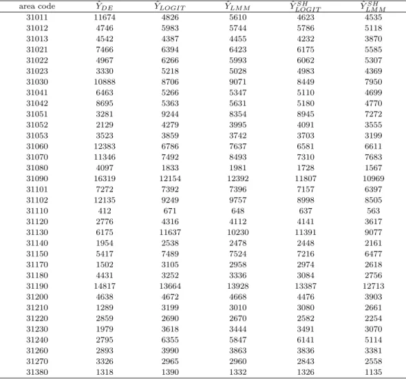
Table 3.1. Estimates of the total number of unemployed persons

area code YˆDE YˆLOGIT YˆLM M Yˆ_LOGIT^SH Yˆ_{LM M}^SH

31011 11674 4826 5610 4623 4535

31012 4746 5983 5744 5786 5118

31013 4542 4387 4455 4232 3870

31021 7466 6394 6423 6175 5585

31022 4967 6266 5993 6062 5307

31023 3330 5218 5028 4983 4369

31030 10888 8706 9071 8449 7950

31041 6463 5266 5347 5110 4699

31042 8695 5363 5631 5180 4770

31051 3281 9244 8354 8945 7272

31052 2129 4279 3995 4091 3555

31053 3523 3859 3742 3703 3199

31060 12383 6786 7637 6581 6611

31070 11346 7492 8493 7310 7683

31080 4097 1833 1981 1728 1567

31090 16319 12154 12392 11807 10969

31101 7272 7392 7396 7157 6397

31102 12135 9249 9757 8998 8505

31110 412 671 648 637 563

31120 2776 4316 4112 4141 3617

31130 6175 11637 10230 11391 9077

31140 1954 2538 2478 2448 2161

31150 5417 7489 7524 7216 6477

31170 1502 3105 2958 2974 2618

31180 4431 3252 3336 3084 2756

31190 14817 13664 13928 13387 12713

31200 4638 4672 4668 4476 3903

31210 1289 3199 3010 3080 2661

31220 2859 2690 2670 2582 2254

31230 1979 3618 3444 3491 3070

31240 2795 6355 5847 6141 5114

31260 2893 3990 3863 3836 3381

31270 3326 2965 2960 2843 2558

31380 1318 1390 1332 1326 1135

Some small areas having all “0” values of the interesting variable are excluded in this analysis.

Therefore, the final data used in this analysis consists of 34 small areas and 4916 observations.

We calculate the sample means and variances in each small area with given samples and obtain the shrinkage estimators. The data set consists of binary response values such as “employed or not”, and the explanatory variable such as administrative district code, gender, level of education, age, and type of housing. Since two variables, level of education(X

1

) and age(X

2

) are statistically significant, we include these two variables as explanatory variables. For 34 small areas, we calculate five small area estimators, ˆ Y

DE

, ˆ Y

LOGIT

, ˆ Y

LM M

, ˆ Y

_LOGIT^SH

and ˆ Y

_{LM M}^SH

with whole data. The results of estimates are shown in Table 3.1.

As mentioned before, the data-based estimator, ˆ Y

DE

is an unbiased estimator; however, it has a

large variance. In several small areas, the estimated values of ˆ Y

DE

are quite different from the other

model based estimates. Especially in small areas coded by 31022, 31060, 31070, ˆ Y

DE

has larger

values than the others. On the contrary, in small areas coded by 31023, 31052, 31120, 31210, the

Table 3.2. Correlation results with ˆYDE

YˆLOGIT YˆLM M Yˆ_LOGIT^SH Yˆ_{LM M}^SH

correlation coefficient 0.75259 0.83137 0.75270 0.82156

results are reversed. The comparison of ˆ Y

LOGIT

with ˆ Y

_LOGIT^SH

shows that all estimates of ˆ Y

LOGIT

are larger than ˆ Y

_LOGIT^SH

as expected. The comparison between ˆ Y

LM M

and ˆ Y

_{LM M}^SH

shows the same phenomena.

In addition, since practically we have no true values of small areas, the comparison of each estimators can be conducted by using the comparison statistics such as regression methods, coverage and calibration. These practically used comparison statistics are studied by Brown et al. (2001). In this study, instead of using those comparison statistics, we simply calculate simple correlation coefficients between ˆ Y

DE

and the other estimators in order to check closeness to ˆ Y

DE

. The results are shown in Table 3.2 and show that ˆ Y

LM M

is better than ˆ Y

LOGIT

. The shrinkage estimators corresponding to the original estimators have almost the same correlation coefficients.

3.2. Simulations

In order to compare the efficiency of these estimators, we conduct a small simulation study. First we select samples without replacement from the whole samples with sample size 2,000, 3,000 and 4,000. We replicate 1,000 times to obtain the comparison statistics. For comparison, five comparison statistics are used. These are Mean Squared Error(MSE), Relative Mean Squared Error(RMSE), Mean Absolute Error(MAE), Absolute Relative Error(ARE), and Relative Bias(RB). Details about these comparison statistics are presented in Rao (2003). Here, Y

i

is the true value for small area i, and each estimate of Y

i

is ˆ Y

i

.

MSE = 1 nR

∑

R r=1

∑

n i=1

( Y ˆ

i,r

− Y

i

)

2

, RMSE = 1

nR

∑

R r=1

∑

n i=1

( Y ˆ

i,r

− Y

i

Y

i

)

2

,

MAE = 1 nR

∑

R r=1

∑

n i=1

  ˆ Y

i,r

− Y

i

  , ARE = 1 nR

∑

R r=1

∑

n i=1

  

Y ˆ

i,r

− Y

i

Y

i

   , RB = 1

nR

∑

R r=1

∑

n i=1

( Y ˆ

i,r

− Y

i

) Y

i

.

Here n = 34 is the number of small areas and R = 1,000 is the number of replications. To use the above statistics, we need to know the true values, Y

i

, i, . . . , n in each small area. However practically we have no true values. So in this simulation, we just assume that the estimates of total in each small area obtained using ˆ Y

DE

with the whole data as the true values shown in Table 3.1.

This is the same way used in Hwang and Shin (2009). The comparison results of estimators are tabulated from Table 3.3 to Table 3.5. Here we drop ˆ Y

DE

in this comparison since only ˆ Y

DE

is a design-based estimator. Notice that MSE and MAE are the statistics about the size of error with RMSE and ARE as the statistics about the size of relative error.

From Table 3.3 to Table 3.5, we have the following results. As expected, values of MSE and MAE of shrinkage estimators, ˆ Y

LOGIT^SH

and ˆ Y

LM M^SH

are larger than those of ˆ Y

LOGIT

and ˆ Y

LM M

respectively.

However, for RMSE and ARE, the values of shrinkage estimators, ˆ Y

LOGIT^SH

and ˆ Y

LM M^SH

have reverse

results. Specially, note that for MSE, ˆ Y

LOGIT

and ˆ Y

_LOGIT^SH

have almost the same results whereas

Table 3.3. Results on comparison statistics with sample size 2,000

MSE RMSE MAE ARE RB(%)

YˆLOGIT 8961892 0.490 2216 0.499 0.232

YˆLM M 7681710 0.347 2004 0.428 0.161

Yˆ_LOGIT^SH 8972775 0.432 2203 0.475 0.178

Yˆ_{LM M}^SH 8317045 0.257 2055 0.39 0.012

Table 3.4. Results on comparison statistics with sample size 3,000

MSE RMSE MAE ARE RB(%)

Yˆ_LOGIT 8472503 0.468 2164 0.491 0.238

Yˆ_{LM M} 6432409 0.273 1814 0.383 0.134

Yˆ_LOGIT^SH 8554284 0.393 2153 0.459 0.167

Yˆ_{LM M}^SH 7418413 0.207 1917 0.356 −0.020

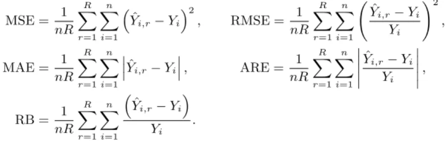
Table 3.5. Results on comparison statistics with sample size 4,000

MSE RMSE MAE ARE RB(%)

YˆLOGIT 8149336 0.448 2126 0.483 0.236

YˆLM M 5566040 0.222 1678 0.348 0.106

Yˆ_LOGIT^SH 8210022 0.393 2119 0.459 0.182

Yˆ_{LM M}^SH 6403534 0.171 1772 0.326 −0.038

Figure 3.1. MSE results

for RMSE, the difference is large. In addition, ˆ Y

LM M

and ˆ Y

LM M^SH

provide the best results in all comparison criteria. For checking unbiasedness, RB is considered and ˆ Y

LM M^SH

shows the best results.

The results show that shrinkage estimators have some bias; however, the values are not large. The shrinkage estimators are shown to produce better results in RB than the corresponding original estimators.

To investigate the trend of magnitude of errors as sample sizes increase, we draw figures of MSE, RMSE, and RB.

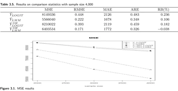
From Figure 3.1 and Figure 3.2, the results on MSE and RMSE, we find that as the sample size increases, ˆ Y

LM M

and ˆ Y

LM M^SH

quickly reduce the magnitude of errors and magnitude of relative errors relatively to ˆ Y

LOGIT

and ˆ Y

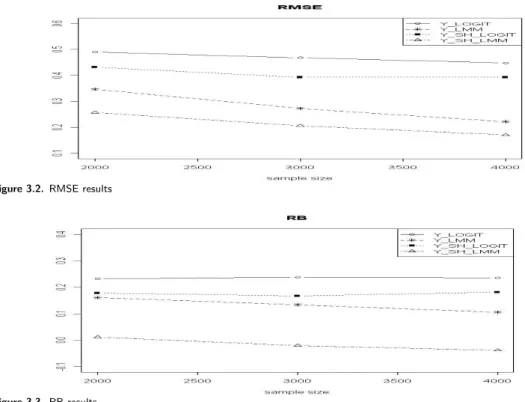
LOGIT^SH

. Figure 3.3, the results on RB, shows that even though ˆ Y

LM M^SH

provide good results, four estimators do not reduce the relative bias as sample size increases.

4. Conclusion

For the small area estimation of binary response data such as un-employment, logistic regression

estimator and logistic mixed estimator are widely used as they have some good statistical proper-

Figure 3.2. RMSE results

Figure 3.3. RB results

ties. These estimators are obtained by minimizing MSE. However, relative error criterion should be considered and applied to obtain the better small area estimation in some cases where the in- terpretation of analysis results is considered as a primary interest rather than the precision of the estimator.

In this paper we study logistic regression type shrinkage estimators obtained by minimizing RE and compare them with logistic regression and logistic mixed estimators. Comparison results based on MSE show that ˆ Y

LM M

is superior to any other estimators including ˆ Y

LOGIT

. However ˆ Y

_{LM M}^SH

shows the best results in RMSE criterion. Therefore we conclude that two small area estimators, Y ˆ

LM M

and ˆ Y

_{LM M}^SH

provide the best results according to proper situations. If an analyst concludes that MSE is a more important criterion than RE, ˆ Y

LM M

should be used; however, in the opposite case, ˆ Y

_{LM M}^SH

should be used.

References

Agresti, A. (2002). Categorical Data Analysis, John Wiley and Son, New York.

Brown, G., Chambers, R., Heady, P. and Heasman, D. (2001). Evaluation of small area estimation meth- ods - Application to unemployment estimations for U.K. L.F.S., Proceedings of Statistics Canada Symposium 2001.

Hwang, H.-J. and Shin, K.-I. (2008). Shrinkage prediction for small area estimations, The Korean Journal of Applied Statistics, 21, 109–123.

Hwang, H.-J. and Shin, K.-I. (2009). A small area estimation for monthly wage using mean squared percent- age error, The Korean Journal of Applied Statistics, 22, 403–414.

Jeong, S. O. and Shin, K.-I. (2008). A new nonparametric method for prediction based on mean squared relative error, The Korean Communications in Statistics, 15, 255–264.

Kim, Y.-W. and Choi, H.-A. (2004). Small area estimation technique based on logistic model to estimate unemployment rate, The Korean Communications in Statistics, 11, 583–595.

Park, H. and Stefanski, L. A. (1997). Relative error prediction, Statistics and Probability Letters, 40, 227–

236.

Rao, J. N. K. (2003). Small Area Estimation, John Wiley and Son, New York.

Yeo, I.-K., Son, K. and Kim, Y.-W. (2008). Small area estimation via generalized estimating equations and the panel analysis of unemployment rate, The Korean Journal of Applied Statistics, 21, 665–674.