Trade-off between Model Complexity and Performance in Intra-frame Predictive Vector Quantization of Wideband Speech

광대역 음성에 대한 프레임내 잔차 벡터 양자화에 있어서 모델 복잡도와 성능 사이의 교환관계

Trade-off between Model Complexity and Performance in Intra-frame Predictive Vector Quantization

of Wideband Speech

송 근 배^†, 한 헌 수¹

Geun-Bae Song^†, Hernsoo Hahn¹

Abstract

This paper addresses a design issue of “model complexity and performance trade-off” in the application of bandwidth extension (BWE) methods to the intra-frame predictivevector quantization problem of wideband speech. It discusses model-based linear and non-linear prediction methods and presents a comparative study of them in terms of prediction gain. Through experimentation, the general trend of saturation in performance (with the increase in model complexity) is observed. However, specifically, it is also observed that there is no significant difference between HMM and GMM-based BWE functions.

Keywords

: Bandwidth Extension, Wideband Speech, Gaussian Mixture Model, Hidden Markov Model

1. Introduction¹⁾

It is well known that there is mutual information between frequency bands in speech

, so a prediction system can be developed to exploit the mutual information. For example, in

, the upper-band information of 4-8 kHz is predicted based on the lower-band information of 0-4 kHz using a codebook mapping and the resulting prediction residual of upper-band is vector quantized (VQ) by a secondary codebook. Test results show that this conditional (or intra-frame predictive) VQleads to a codinggain of appro- ximately 1 bit over a simple VQ. Similar approach also can

Received: Jan. 29, 2010; Reviewed: Jan. 29, 2010; Accepted: Feb. 01, 2010

※ This research was supported by the MKE (The Ministry of Knowledge Economy), Korea, under the ITRC (Information Technology Research Center)program supervised by the NIPA (National IT Industry Promotion Agency) (NIPA-2009-(C1090-0902-007))

※ This work was supported by the Korea Research Foundation Grant funded by the Korean Government (MOEHRD).

† ITRC, Soongsil Univ. ([email protected])

1 School of Electronics Engineering, Soongsil Univ. ([email protected])

be seen in

, where Geiser et al. employ a linear mapping function for the same purpose and reports a good performance satisfying the target bit-rate of 400 bps.

So far, various estimation functions that exploit the mutual information between frequency bands have been developed in the area of bandwidth extension (BWE) [4]. All of them could be classified into three categories: (1) linear mapping, (2) codebook mapping, and (3) hidden Markov model (HMM) based mapping. In particular, the codebook mapping canbe represented by the Gaussian mixture model (GMM) based mapping since this algorithmallows for much more flexible clustering than the conventional hard-classification ones

. It is shown in

that the HMM framework has certain parallels with all other existing functions under proper conditions, and thus, roughly, it could be said that the HMM method is the most generalized mapping function and perform at least not worse than other functions (at the cost of higher complexity).

In this paper, we are interested in further investigating the

prediction scheme for efficient representation or low bit-rate

BWE

Channel

( ) m x

( ) m VQ

y +

−

( ) m

r r ˆ( ) m

( ) m y%

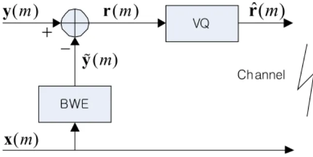
Fig. 1. Intra-frame predictive vector quantization scheme

coding of the upper-band signals. First, we briefly summarize the three representative prediction functions that have been mentioned above, and present a comparative study of them to see how well they exploit the mutual information (also called here intra-frame correlation). This paper is organized as follows. In Section 2, an explanation of the intra-frame predictive VQ is given as well as a discussion of Mel-frequency cepstral coefficients (MFCCs) parameterization.

In Section 3, the three representative mapping functions are briefly reviewed, as well as the factthat the GMM-based function can be considered as a special case of HMM-based function with a single state. In Section 4, the general trend of model complexity and performance trade-off and the limitation of complex non-linear function are discussed through experimentation. Finally, Section 5 concludes the paper.

2. Intra-frame predictive VQ

2.1 Parameterization

In general, it is acknowledged that the human ear is insensitive to distortions of the excitation signal at high frequencies above 3.4 kHz and the spectral envelope informationis more important for the subjective quality [4].

Therefore, main concern could be laid on encoding the spectral envelope and spectral energy information. In this work, MFCC coefficients are used for parameterization of speech signals. They are known to be the best in terms of the total score of mutual information and separability compared to other popular parameters such as line spectral frequencies (LSFs) or linear prediction coefficients (LPCs)

, and, thus, more suitable for BWE problem. Moreover, they can be equivalently transformed to (perceptually-weighted!) LPC coefficients, so usable for speech reconstruction in the decoder

(see [4] or [6]).Accordingly, without significant loss of generality, we use this parameterization for the representation of speech signals.

In the wide-band range of 0-8 kHz, the band of 3.7-8 kHz is defined as upper-band, and represented by fifth-order MFCCs:

0 1 4

[ , ,..., ] y y y

=

y , (1)

where T denotes the transpose operation. The lower-band of 50 Hz-3.7 kHz which can be filled with fifteen Mel-scale filters is represented by the fifteen MFCCs:

0 1 14

[ , ,..., x x x ]

=

x . (2)

Note here that the zero-order parameters of y

and x

corresponds to the logarithmic energy of respective frequency bands.

2.2 Intra-frame prediction and VQ

As mentioned, the advantage of intra-frame predictiveVQ over other VQ methods is achieved mainly by exploiting a statistical dependency between frequency bands. Let x be the lower-band vector, and y and y% , respectively, be the upper-band and estimated upper-band vectors, then the residual vector at the mth frame is calculated as follows:

( ) m = ( ) m − ( ) m = ( ) m − { ( )} m

r y y % y F x , (3)

where F{·s a mapping function (or BWE function) that exploit the statistical dependency between x(m) and y(m).

Generally, the variance of the residual vector, r(m), is smaller than that of the original vector, y(m), so some coding gain can be achieved with this approach. The VQ codebook that is used to vector quantize the residual signals is trained using the well-known LBG algorithm

.

3. Representative BWE functions

3.1 Minimum mean square error estimation rule

The error criterion that is minimized by the minimum

mean square estimation (MMSE) rule is the mean square

error, as follows:

{ ( ) ( ) | ( )}

MSE

E m m m

ε

= y − y % Ξ ^{, (4)}

where E{·}denotes the expectation with respect to the underlying distribution of y(m) and ||·| denotes the Euclidean norm. In addition, Ξ ( ) m = { (1), (2),..., ( )} x x x m _denotes the sequence of lower-band vectors observed up to the mth frame.

3.2 Linear function

If a linear function is used, then F{·}can be represented by the following transformation matrix:

( ) m =

( ) m

y % H x ^{, (5)}

and the transformation matrix H is computed by the least squares method as follows:

(

)

=

H X X X Y , (6)

where the rows of matrix X consist of all the lower-band training vectors and the rows of matrix Y consist of all the upper-band training vectors that one-to-one correspond to the respective row vectors of matrix X. Accordingly, let M be the total number of vectors, then the size of X is Mx15, and that of Y is Mx5.

If a sequence of vectors are stationary and ergodic, then the time-averaged distortion,

2 0

1

( ) m ( ) m

M ∑

^y − ^{y% , (7)}

converges with probability one to the mean square error

as M → ∞ (from the ergodic theorem), that is,

describes the long-run time-averaged distortion. In this case, the least squaresestimation rule is equivalent to the MMSE estimation rule.

3.3 Non-linear functions

In this section, we review the MMSE estimation rule that utilizes the trained HMM models, as well as the relation between HMM and GMM. Further details on this topic can be found in [4] or [8]. Given a statistical model of wideband

speech, the estimation rule for upper-band information can be designed based on the MMSE criterion of Eq. (4):

*

* 2

( ) arg min { ( )

( ) | ( )}

m =

E m − m m

y

y y Ξ

%

% . (8)

It is well known that the solution of Eq. (8) is the conditional expectation called the MMSE estimation rule:

y % ( ) m = E { ( ) | ( )} y m Ξ m

( ) ( ( ) | ( )) ( ) m p m m d m

= ∫

y y Ξ y _{. (9)}

Now, with some manipulations on the conditional density function p ( ( ) | ( )) y m Ξ m utilizing the states of HMM model, Eq. (9) can be modified to be a weighted sum of component-wise conditional expectations:

1

( )

( ( ) | ( )) { ( ) | ( ), ( )}

N

i i

i

m P S m m E m S m m

=

= ∑

y % Ξ y x , (10)

where N

denotes the total number of states in the HMM model, and S

(m) means that the state of the mth frame is i.

In particular, this estimation rule is called as the “cascaded estimation” rule by Jax, since first the conditional expectation E{y(m)| S

(m), x(m)} is calculated for each state, followed by an individual weighting with the respective a posteriori probabilities, P S m ( ( ) | ( ))

Ξ m . Jax also tested a few other types of estimation rules under the same MMSE criterion. In conclusion, the cascaded estimation rule is the most general function of the testedrules with the highest computational complexity, thus it is shown to produce the highest performance.

On the other hand, the weighting probability ( ( ) | ( ))

P S m Ξ m is related to the dynamic modeling ability

of HMM model since its calculation needs the state

parameters of HMM model as well as the observation

parameters. But, the conditional expectation E{y(m)| S

(m),

x(m)} needs only the observation parameters and, thus,related

only to the static modeling ability of HMM model. As the

number of states increases, the weighting probability will be

gradually refined and the dynamic performance of the

estimation rule becomesbetter, while this performance will be

worse as the state number decreases. As an extreme case, if

the number decreases to a single state, e.g., S

, then the weighting probability becomes P S m ( ( ) | ( )) 1

Ξ m = , and Eq.

(10) reduces to the simple conditional expectation,

y % ( ) m = E { ( ) | , ( )} y m S

x m { ( ) | ( )}

E m m

= y x . (11)

Generally speaking, this expectation is an MMSE estimation rule that minimizes the following criterion:

*

* 2

( ) arg min { ( )

( ) | ( )}

m =

E m − m m

y

y y x

%

% , (12)

where, comparing with Eq. (8), it can be known that the conditional observation has been changed from the sequence

( ) m

Ξ (up to the mth frame) to the vector x(m) at the mth frame. As mentioned previously, this conditional expectation needs only the observation parameters of HMM model (with a single state). Therefore, it can be easily understood that the HMM-based estimation rule reduces to the GMM-based estimation ruleif the HMM model employs a single state and the GMM-based observation density function. If the covariance matrix of GMM model is diagonal, then the GMM-based estimation rule (or the conditional expectation of Eq. (11)) can be simply represented as follows:

{ ( ) | ( )} ( )

( ( ) | ( )) ( ) E y m x m = ∫

y m p

y m x m d m y

, , , ,

1

, , ,

1

( ( ); , ) ( ( ); , )

L

l l l l

l L

l l l

l

f m f m

ρ

=

=

= ∑

∑

x x x y

x x x

x μ V μ

x μ V ^{, (13)}

where L is the number of GMM components,

_, μ

_{, and}

,l

V

, respectively, denote the prior, the mean vector, and the (diagonal!) co-variance matrix of the lth GMM component for lower-band vector. In addition, μ

denotes the mean vector of the lthGMM component for the upper-band vector. This expression is directly derived from the full co-variance case of Eq. (6) of [5], if the cross-covariance matrix between vectors x and y (denoted C

in the paper) is set to be the zero matrix from the ‘diagonal’ assumption.

A single and large ergodic HMM is trainedto represent the

statistical characteristic of wide-band training data, where the

‘ergodic’ means that the transition from any state to any other state shall be possible. The covariance matrix of GMM model is approximated with the diagonal matrix since different MFCC coefficients are near uncorrelated. The general Baum-Welch algorithm is used to train the HMM model, starting with VQ initialization as usual (refer to [6] for more details).

4. Performance evaluation

4.1 Training data and performance measures The 16 kHz-sampled TIMIT database is used for training and testing [9]. In training, the whole training set (462 speakers, total 4620 utterances) is used, while only the core test set (24 speakers, total 192 utterances) defined in TIMIT is used for testing. The utterances are windowed using a 20ms Hamming window without over-lap, and then MFCC coefficients are extracted from the resulting frames.

The prediction gain (PG) that is the ratio between signal energy and prediction-error energy is used for testing the performance of prediction methods. It is defined as:

(

)

10 log

( ) ( )

BWE m m

PG = ∑ ^y m ∑ ^r m [dB]. (14)

In addition, as a measure for testing quantization performance, the Euclidean cepstral distance between the original and quantized vectors is used, given by:

2

( ) ( ) ˆ ( )

d

m = y m − y m [dB]. (15)

As well known [1], [4], this measure is directly related to the log spectral distortion (LSD) that is commonly used in the area of speech coding:

4 2

2 2

10 0

( ) 1 20 log ˆ

5 ( )

E cep

k E

d H k LSD

H k

=

⎛ ⎞

= ⎜ ⎟ ≈

⎝ ⎠

∑ _{, (16)}

where H

_and ˆ

H

, respectively, denotethe original and

quantized Mel-warped spectral envelops. (Note that the frame

index m is omitted for brevity.)

GMM HMM

Linear

1x64 1x128 1x256 64x1 128x1 256x1

4.59 4.86 5.13 4.53 4.77 5.03 3.79

Table 1. Prediction gain (in dB) of different GMM and HMM configur- ations, and linear mapping function

1 x L (GMM)

BWE PG [dB]

70 60 50 40 30 20 10 0 4.5

4.0

3.5

3.0

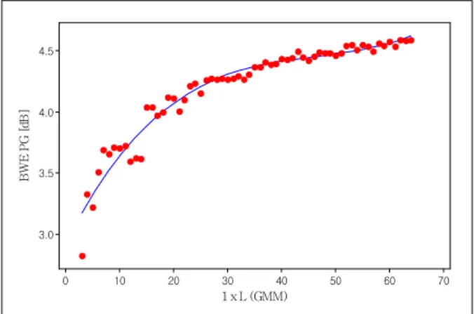
Fig. 2. BWE prediction gain w.r.t. complexity of GMM function

4.2 Mutual information measurements

The mutual informationmeasurements for six different sound classes such as fricatives or vowels are given in [1], where they are ranged from 1.09 to 1.60 bits. Although we can calculate the total average (i.e., 1.35 bits) from this data, this average value does not reflect the difference between distributions of the classes. Therefore, we re-calculated it using the TIMIT data and with the procedure as in [1]. As a result, it was measured a little higher than the above value.

For example, for three different cases of GMM model, i.e., for the total Gaussian number L= 64, 128, and 256, it is measured 1.44, 1.56, and 1.69 bits, respectively. It is interesting that, as model complexity increases (i.e., better fitted to training data), the value increases slightly. So, considering this tendency, roughly it could be stated that the mutual information of wideband speech (based on MFCCparameterization) is near or a little less than 2 bits.

4.3 Test results in terms of prediction gain As a conclusion, we found that the performance of HMM method depends only on the total number of Gaussian components of HMM model, but not on any specific configuration of the model. For example, for the total Gaussian number of N

xL=64 (where N

is the number of states and L is that of Gaussian components of each state), the HMM configurations such as 64x1, 32x2, 16x4, or even 1x64 (i.e., GMM) appeared to have almost the same performance. Therefore, only the maximum-state cases such as 64x1 or 256x1 are considered here as the HMM configuration. Table 1 shows the prediction gain of a few configurations of HMM and GMM functions, as well as the result of linear function. As mentioned, the difference between HMM and GMM is marginal for the same number of N

xL, but they outperform explicitly the linear mapping. Roughly, the GMM configuration of 1x9 (of which PG is 3.71 dB) is observed to be fairly comparable with the performance of linear mapping. An important advantage of linear mapping is its simplicity. That is, it requires 15x5=75 multiplications for

each frame (refer to the matrix operation of Eq. (5)), while the GMM function can realize this low complexity under the very simple configuration of 1x2 (refer to Eq. (13)). The HMM function is basically more complex than the GMM function since it needs an additional computation of state probabilities, i.e., the weighting probability P S m ( ( ) | ( ))

Ξ m of Eq. (10). It is also interesting to note that, even though marginal, the GMM function consistently outperforms the HMM function for all cases, as seen in the table. This seems to be caused from the local maxima problem of HMM training. That is, as the model complexity increases, the fully-connected HMM topology is more likely to get trapped in local maxima compared to the relatively simple GMM method, thus leading to relatively sub-optimal results.

To get a comprehensible indication of a relation of prediction gain and (BWE) complexity, it would be helpful to draw a scatter plot of them. For the purpose, various PG values have been computed by changing the configuration of GMM model from N

xL=1x3 to 1x64 (62 cases in total). Fig.

2 shows the values of prediction gain against the configuration of GMM model. It is observed in the figure that the prediction gain consistently increases with the configuration complexity, but the gain gradually saturates around the configuration of 1x30. In the end, the saturation limit will be determined by the mutual information between frequency bands.

As a conclusion, although the linear prediction is very attractive in terms of computational complexity, it is also confirmed that the GMM (or HMM) function explicitly outperforms the linear mapping with increased complexity.

Therefore, these non-linear functions could compete with the

linear mapping in the applications where the complexity requirement is not too strict.

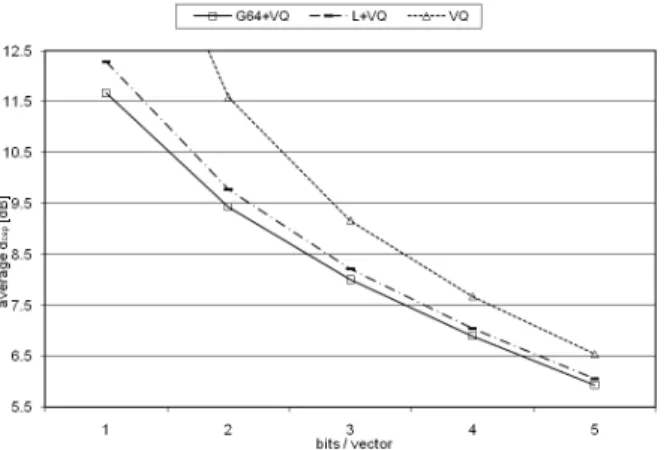
4. 4 Test results of different VQ schemes Finally, the vector quantizer is integrated with the intra-frame predictive scheme and the quantization results of respective BWE functions are compared in terms of Euclidean cepstral distance. In Fig. 3, ‘G64+VQ’ and ‘L+VQ’, respectively, denote the 1x64 GMM function and the linear function, each combined with respective VQs. The results for HMM are omitted here since they are almost the same as those of the corresponding GMM cases. For reference, the results for simple VQ are also given in the figure.

Overall results are consistent with the observations in the previous section. It is explicit that the combination of intra-frame predictive scheme with the VQ is beneficial for overall quantization performance. The GMM function consistently outperforms the linear function for all cases, and it is also show this difference decreases as the bit-rate increases.

Fig. 3. Performance comparison of intra-frame predictive VQs and simple VQ w.r.t. bit-rate.

5. Conclusion

In the application BWE techniques to the intra-frame predictive VQ problem of wideband speech, more complex statistical algorithms could compete with the simplest linear mapping as a tradeoff between efficiency and complexity. It is shown that the improvement in performance saturates with the increase in model complexity, in particular at around the configuration of 1x30. This graph agrees with the general

tendency of saturation in performance. The comparison of GMM and linear function says that the non-linear approach could compete with the linear mapping in some applications where the complexity requirement is not too strict. However, it is observed that there is no significant difference between HMM and GMM BWE functions.

Within the scope of this paper, the optimization problem of VQ system has not been elaborately examined, and further work is required to improve it in conjunction with the intra-frame predictive scheme.

참 고 문 헌

[1] M. Nilsson, H. Gustafsson, S. Andersen, and W.

Kleijn, “Gaussian mixture model based mutual information between frequency bands in speech,”

ICASSP, Vol.1, pp.525-528, May 2002.

[2] Y. Agiomyrgiannakis and Y. Stylianou, “Conditional vector quantization for speech coding,” IEEE Trans.

Audio, Speech, Lang. Process., Vol.15, No.2, pp.377- 386, Feb. 2007.

[3] B. Geiser and P. Vary, “Backwards compatible wideband telephony in mobile networks: CELP watermarking and bandwidth extension,” ICASSP, Vol.4, pp.533-536, April 2007.

[4] P. Jax, “Bandwidth extension for speech,” in Audio Bandwidth Extension, E. Larsen and R. M. Aarts (Ed.), NY:John Wiley & Sons, Nov. 2004, Chap. 6, pp.171-235.

[5] K. -Y. Park, H.S. Kim, “Narrowband to wideband conversion of speech using GMM based transformation,”

ICASSP, Vol.3, pp.1843-1846, June 2000.

[6] G. -B. Song and P. Martynovich, “A Study of HMM-based bandwidth extension of speech signals,”

Signal Processing, Vol.89, No.10, pp.2036-2044, Oct.

2009.

[7] Linde Y, Buzo A, and Gray RM, “An algorithm for vector quantizer design,” IEEE Trans. Comm. Vol.28, No.1, pp.84-95, 1980.

[8] P. Jax, and P. Vary, “Artificial bandwidth extension

of speech signals using MMSE estimation based on a

hidden Markov model,” ICASSP, Vol.1, pp.680-683,

April 2003.

[9] J. S. Garofolo, L. F. Fisher, J. G. Fiscus, D. S.

Pallett, and N. L. Dahlgren, “DARPA TIMIT Acoustic- Phonetic Continuous Speech Corpus CD-ROM,”

NIST, 1990.

Geun-Bae Song received the B. S., M. S., and Ph. D.

degrees in Electronics Engine- ering at Ajou University, Korea, in 1992, 1995, and 2001, respectively. He is currently a Post-doctoral researcher in Intelligent Robot Research Center at Soongsil University.

His research interests include speech signal processing and pattern recognition.

Hernsoo Hahn received the B. S. and M. S. degrees in Electronics Engineering at Soongsil University and Younsei University, Korea, in 1982 and 1983, respectively. He received the Ph. D degree in Computer Engineering from University of Southern California in 1991, and became an Assistant Professor at the School Electronics Engineering in Soongsil Universityin 1992.

Currently, he is a Professor. His research interests include

application of vision sensors to mobile robots and

measurement systems.