New Wald Test Compared with Chen and Fienberg's for Testing Independence in Incomplete Contingency Tables

(1)

2005, Vol. 16, No. 1, pp. 137∼144

New Wald Test Compared with Chen and Fienberg's for Testing Independence in Incomplete Contingency

Tables

Shin-Soo Kang¹⁾

Abstract

In I× J incomplete contingency tables, the test of independence proposed by Chen and Fienberg(1974) uses I×J - 1 instead of ( I - 1)( J - 1 ) degrees of freedom without providing much of an increase in the value of the test statistic. For these reasons, Chen and Fienberg tests are expected to have less power. New Wald test statistic related to the part of Chen and Fienberg test statistic is proposed using delta method.

These two tests are compared through Monte Carlo studies.

Keywords : Complete Case Analysis, MLE, Wald Statistic

1. Introduction

In the analysis of contingency tables, it may happen that some observations are fully classified or others are partially classified. These tables are called

`incomplete contingency table'.

Blumenthal (1968) considered two way contingency tables for multinomial samples where the column classification is missing. Chen and Fienberg (1974) used an iterative procedure for computing maximum likelihood estimates and developed Pearson and likelihood ratio tests of independence for two-way tables for which either the row or column classification could be missing for some cases. As in Chen and Fienberg (1974), Hocking and Oxspring (1974) consider three independent multinomial distributions corresponding to the set of fully cross-classified counts and the two sets of partially classified counts, where either the row classification or the column classification is missing.

1) Professor, Department of Information Statistics, Kwandong University, Kangnung, 210-701, Korea

E-mail: [email protected]

(2)

cases are completely classified, by imputing information for the missing row or column classification. Multiple imputation, proposed by Rubin (1978), provides a way to take advantage of common tests of independence for completely classified tables.

Little and Rubin (2002) in Section 1.3 discussed three general mechanisms for missing data: missing completely at random(MCAR), missing at random(MAR), and not missing at random(NMAR). Let X₁ and X₂ denote categorical variables for a two-way incomplete contingency table. If the missing probability of Xi

does not depend on either the value of the other variable or the value of Xi, then it is MCAR. If the missing probability of X_i depends on the value of the other variable but not on the value of Xi, then it is MAR. If the missing probability of Xi depends on its value, then it is NMAR.

The proposed new Wald tests of independence in Section 4 and the tests derived by Chen and Fienberg(1974) are examined through Monte Carlo studies in Section 5 considering both type I error level and power.

2. Notation and MLE under independence model

Consider an I× J contingency table where the row factor X₁ has I categories and the column factor X2 has J categories. Assume simple random sampling with replacement. In a complete table, where the row and column categories are observed for every case in the sample, the counts have a multinomial distribution with sample size N and probability vector θ, where θ = ( θ₁₁,θ₁₂,…θ_1J,θ₂₁,…,…,θ_IJ). Let n_ij denote the count for the cell ( i,j), and let θij, an element of θ, denote the population proportion for the cell (i,j).

When information on either the row or column classification is missing, we can construct a table of counts for the completely classified cases where xij denotes the number of cases observed in the ( i,j) cell. We can also construct one-way tables of counts for partially classified cases. Let xim denote the number of cases in the i^th row category, i = 1,2,…,I, where the column category is unknown, and let xmj denote the number of cases in the j^th column category, j = 1,2,…,J, where the row category is unknown. Then, x_im and xmj are marginally observed counts on a single variable. Let x_mm denote the number of cases where both the row and column categories are missing. The total sample size is

(3)

N = ∑

ijx_ij+∑

i x_im+∑

j x_mj+ x_mm

= n_cc+x_{+ m}+x_{m +}+x_mm.

The likelihood function for the observed counts assuming MCAR or MAR is proportional to

[^{i = 1}^∏Î ^{j = 1}^∏^J ^θ îj^xîj][^{i = 1}^∏Î ^θ^{i +}^xîm][^{j = 1}^∏^J ^θ^{+ j}^x^mj]^.

The MLE's of { θ_ij} under independence model proposed by Chen and Fienberg(1974) are θˆ

ij=( ⁿ^x^cc^{i +}^+x^{+ x}^{+ m}^im )( ⁿ^x^cc^{+ j}^+x^{+ x}^{m +}^mj )^, i = 1,2,…,I and j = 1,2,…,J.

3. Chen and Fienberg Test

The test proposed by Chen and Fienberg(1974) consists of three parts, one is essentially a test for independence for the fully observed data and the other two correspond to tests for row and column margins, respectively:

X²= ∑

I i = 1 ∑

J j = 1

(x_ij- αˆ

ij)² ˆα

ij

+ ∑

I i = 1

(x _im- βˆ

i)² ˆβ

i

+ ∑

J j = 1

(x_mj- σˆ

j)² ˆσ

j

, (1)

where ˆα

ij, βˆ

i and σˆ

j are the expected values under independence model assuming MCAR such as

ˆα

ij = n_cc( ⁿ^x^cc^{i +}^+x^{+ x}^{+ m}^im )( ⁿ^x^cc^{+ j}^+x^{+ x}^{m +}^mj )^,

ˆβ

i = x_{+ m}( ⁿ^x^cc^{i +}^+x^{+ x}^{+ m}^im )^,

ˆσ

j = x_{m +}( ⁿ^x^cc^{+ j}^+x^{+ x}^{m +}^mj )^.

If the missing mechanism does not satisfy missing completely at random(MCAR) criterion, there is no explicit form for the expected values in (1).

We require iteration procedure to get the expected values.

The last two parts in (1), for partially classified counts, do not provide much

(4)

parts, for partially classified counts, are close to central Chi-square distributions even though the null hypothesis of independence is not true. The test statistic in (1) uses I×J - 1 instead of (I -1)( J-1) degrees of freedom without providing much of an increase in the value of the test statistic. For these reasons, Chen and Fienberg tests are expected to have less power.

4. New Wald test

Let C₀= ( x₁₁,…,x_1J,x₂₁,…,x_2J,…x_IJ,x_m1,…,x_mJ,x_1m,…x_Im)^'. Conditional on the value of x_mm, C₀ has a multinomial distribution with sample size

n= N- x_mm and probabilities

π = ( π ₁₁,…,π_1J,π₂₁,…,π_2J,…π_IJ,π_m1,…,π_mJ,π_1m,…π_Im)^'.

The expected counts for the fully classified counts are n_ccˆθ

ij. The differences between the fully classified counts and the expected counts under independence model are

a_ij= x_ij- n_cc( ⁿ^x^cc^{i +}^+x^{+ x}^{+ m}^im )( ⁿ^x^cc^{+ j}^+x^{+ x}^{m +}^mj )^.

The variance-covariance matrix of C0 is Var( C₀) = n(^Δπ- ππ^')≡V, where Δ_π is a diagonal matrix with the elements of π on the main diagonal. For I× J tables, let A^'= ( a₁₁,…,a_1J,a₂₁,…,a_2J,…a_IJ)^', then Var(A) = DVD^'≡Σ_a, where D is the matrix of the first partial derivatives of A with respect to x's in C₀ as follows:

D _p×q= ꀌ

ꀘ

︳︳

︳

ꀍ

ꀙ

︳︳

︳

∂a₁₁

∂x₁₁ … ∂a₁₁

∂x_IJ

∂a₁₁

∂x_m1 … ∂a ₁₁

∂x_mJ

∂a₁₁

∂x _1m … ∂a₁₁

∂x _Im

∂a₁₂

∂x ₁₁ … ∂a₁₂

∂x _IJ

∂a ₁₂

∂x_m1 … ∂a ₁₂

∂x_mJ

∂a₁₂

∂x _1m … ∂a₁₂

∂x_Im

⋯ ⋯ ⋯

∂a _IJ

∂x₁₁ … ∂a_IJ

∂x _IJ

∂a _IJ

∂x_m1 … ∂a _IJ

∂x _mJ

∂a_IJ

∂x _1m … ∂a_IJ

∂x _Im ,

where p = I×J and q = I×J + I + J.

(5)

Let Ri= r_i

r₊ =( ⁿ^x^cc^{i +}^+x^{+ x}^{+ m}^im )^{and C}^j⁼ ^c^c⁺^j ⁼( ⁿ^x^cc^{+ j}^+x^{+ x}^{m +}^mj ), then the elements of D matrix are

∂a _ij

∂x_cd = ꀊ

ꀖ ꀈ

︳︳

︳

︳︳

︳

1 - R_iC_j-n_cc(^C^j ^r⁺^r^-r²⁺ ⁱ^{+ R}ⁱ ^c⁺^c^-c²⁺ ^j ), c = i,d = j - R_iC_j- n_cc(^C^j ^r⁺^r^-r²⁺ ⁱ ^{- R}ⁱ^c^c²⁺^j )^, c = i,d≠j,d≠m - R_iC_j- n_cc(^C^j^-r^r²⁺ⁱ ^{+ R}ⁱ ^c⁺^c^-c²⁺ ^j )^, c≠i,d = j,c≠m - n_cc(^Rⁱ ^c⁺^c^-c²⁺ ^j )^, c = m,d = j - n_cc(^Rⁱ^-^c^c²⁺^j )^, ^{c = m,d≠j}

- n_cc(^C^j ^r⁺^r^-r²⁺ ⁱ )^, c = i,d = m - n_cc(^C^j^-^r^r²⁺ⁱ )^, ^{c≠i,d = m}

- R_iC_j- n_cc(^C^j^-^r^r²⁺ⁱ ^{+ R}ⁱ^-^c^c²⁺^j )^, c≠i,d≠j,c≠m,d≠m.

The hypothesis of independence for I× J tables is {^H^H⁰¹^{:E( A) = 0}^{:E( A)≠ 0.} The Wald statistic to test of independence is A^' ˆΣ_a^-A and this test statistic has an asymptotic χ² distribution with I×J - 1 degree of freedom. π is evaluated using sample proportion to estimate Σ_a

5. Simulation Study

The proposed test in Section 4 is compared with the Chen and Fienberg(1974) test through Monte Carlo simulations. For each combination of sample size and level of missingness, Type I error levels are estimated from 1,000 simulated tables under the independence assumption. Power levels are examined by simulating 1000 tables under an alternative to independence.

(6)

5.1 Type I error levels

All of the 2× 2 incomplete contingency tables to check Type I error levels were generated with equal cell probabilities and data missing completely at random.

Four combinations of sample size and level of missing data were considered and 1000 tables were generated for each combination. X₁ and X₂ were independently generated from Bernouli(0.5) random variables. There are two levels N=200 and N=400 for the total sample size N. MX_i is a missing indicator variable independent of Xi. If MXi= 1, the corresponding variable X_i is missing. The four combinations of factors are summarized in Table 1. The percentages of cases with missing information on at least one variable are expected to be 19%, 36%, 51%, and 91% for combination 1, 2, 3, and 4, respectively.

Table 1: Combination of factors generated to check Type I error levels MX_i∼Ber( p)

Combination N p

1 200 0.1

2 200 0.2

3 200 0.3

4 400 0.7

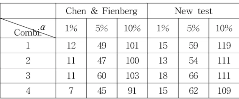
Table 2 shows the numbers of tables for which the independence null hypothesis was falsely rejected out of 1000 tables for three nominal Type I error levels. The results of two methods seem to have appropriate Type I error levels but the new method has more inflated Type I error levels than Chen and Fienberg test in all combinations.

Table 2: Comparison of Type I error levels Chen & Fienberg New test α

Combi. 1% 5% 10% 1% 5% 10%

1 12 49 101 15 59 119

2 11 47 100 13 54 111

3 11 60 103 18 66 111

4 7 45 91 15 62 109

(7)

5.2 Power Study

There are 4 alternatives to independence for 2× 2 tables with equal probability margins to check power. The generated multinomial variables have the cell probability such that

( θ₁₁,θ ₁₂,θ₂₁,θ₂₂)= (0.2,0.3,0.3,0.2) for all combinations in Table 1.

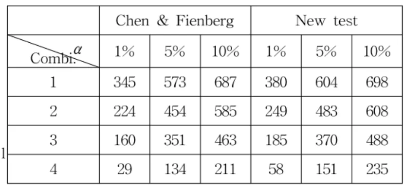
The numbers in Table 3 indicate the number of tables out of 1000 for which the independence null hypothesis was rejected under the given α levels among 1000 tables in each combination.

Table 3 shows new method has more power than Chen and Fienberg test. As the proportion of missing cases increases from 19% to 91%, the power decreases as expected.

Table 3: Power Comparison

l

Chen & Fienberg New test α

Combi. 1% 5% 10% 1% 5% 10%

1 345 573 687 380 604 698

2 224 454 585 249 483 608

3 160 351 463 185 370 488

4 29 134 211 58 151 235

6. Conclusion

Chen and Fienberg‘s test is more conservative and has less power in most cases than new Wald test. If there are lots of missing values, we can expect that new test has more appropriate Type I error level and more power.

If the missing mechanism does not satisfy missing completely at random(MCAR) criterion, Chen and Fienberg test statistic has no explicit formula. The Wald test proposed in Section 4 also works under MAR missing mechanism.

(8)

References

1. Blumenthal, S. (1968). Multinomial sampling with Partially Categorized Data, Journal of the American Statistical Association, 63, 542-551.

2. Chen, T. T., and Fienberg, S. E. (1974). Two-dimensional contingency tables with both completely and partially cross-classified data,

Biometrics, 32, 133-144.

3. Hocking, R. R., and Oxspring, H. H. (1974). The Analysis of Partially Categorized contingency Data, Biometrics, 30, 469-483.

4. Little, R. J. A., and Rubin, D. B. (2002). Statistical analysis with missing data, J. Wiley and Sons, New York.

5. Rubin, D. B. (1978). Multiple Imputation in Sample Surveys - A Phenomenological Bayesian Approach to Nonresponse, Proceedings of the Survey Research Methods Section, American Statistical Association, 1978, 20-34.

[ received date : Sep. 2004, accepted date : Dec. 2004 ]