published first issue April 2013 J
1. INTRODUCTION
The global positioning system (GPS) refers to a system which can precisely trace a user position using the signal from the satellite, and is currently utilized in various fields.
For the signal from the satellite, a delay occurs before reaching the user while passing through the ionosphere and troposphere, which causes an error in the user position.
Therefore, diverse models have been developed to correct this error. The ionospheric delay error changes significantly by the solar activity, and has a large variation depending on location. For the last 20 years, many studies have been performed to precisely model the ionosphere which has the above-mentioned characteristics, and the studies are also currently in progress. Depending on purpose, the ionosphere model can be divided into the real-time model
Performance Evaluation of Ionosphere Modeling Using Spherical Harmonics in the Korean Peninsula
Deokhwa Han
†, Ho Yun, Changdon Kee
School of Mechanical and Aerospace Engineering and SNU-IAMD, Seoul National University, Seoul 151-744, Korea
ABSTRACT
The signal broadcast from a GPS satellite experiences code delay and carrier phase advance while passing through the ionosphere, which causes a signal error. Many ionosphere models have been studied to correct this ionospheric delay error.
In this paper, the ionosphere modeling for the Korean Peninsula was carried out using a spherical harmonics based model.
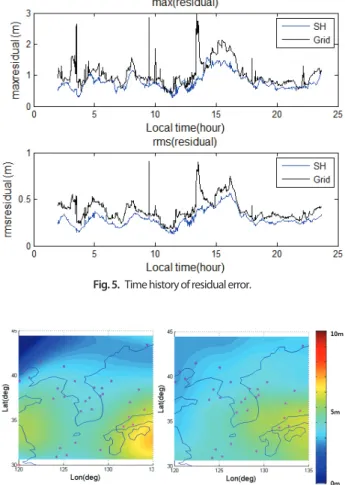
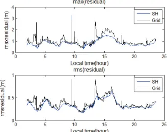
In contrast to the previous studies, we considered a real-time ionospheric delay correction model using fewer number of basis functions. The modeling performance was evaluated by comparing with a grid model. Total number of basis functions was set to be identical to the number of grid points in the grid model. The performance test was conducted using the GPS measurements collected from 5 reference stations during 24 hours. In the test result, the modeling residual error was smaller than that of the existing grid model. However, when the number of measurements was small and the measurements were not evenly distributed, the overall trend was found to be problematic. For improving this problem, we implemented the modeling with additional virtual measurements.
Keywords: GPS, ionosphere, spherical harmonics
for providing the correction information to user in real time, and the post-processing model for various research purposes. The representative real-time models are the Klobuchar model which is currently broadcast from GPS satellites by being included in the navigation data, and the grid model which is used for the Wide Area Differential GPS (WADGPS) such as the Wide Area Augmentation System of the United States. The post-processing models are the Global Ionospheric Map model which provides the latitude and longitude of the entire globe by dividing into a grid of 2.5° × 5°, and the International Reference Ionospheremodel (Choi et al. 2010).
In this paper, the ionosphere modeling for the Korean Peninsula was carried out using spherical harmonics.
A number of studies have already been performed regarding the ionosphere modeling using spherical harmonics (Choi et al. 2010, Moon 2004, Venkata Ratnam et al. 2009). However, most previous studies have used spherical harmonics for the post-processing model, and the performance has not been evaluated when spherical harmonics are used for the real-time ionospheric correction Received Mar 29, 2013 Revised Apr 28, 2013 Accepted Apr 29, 2013
†
Corresponding Author E-mail: [email protected]
Tel: +82-2-880-7395 Fax: +82-2-878-0559
model. In this paper, the spherical harmonics ionosphere modeling was performed which appropriately adjusted the number of basis functions considering the real-time ionospheric correction, and assuming that the model is used for WADGPS, the performance was tested by comparing with the grid model which is currently in use.
The actual data collection and Differential Code Bias (DCB) estimation procedure were conducted in a post-processing way, and the modeling was performed using the obtained ionospheric delay measurement.
2. IONOSPHERIC DELAY MEASUREMENT
The signal transmitted from a satellite passes through the atmosphere before reaching the user. In the upper atmosphere, gas molecules are ionized by the effect of ultraviolet rays and exist as the plasma state which has a high density of free electrons. This region is called ionosphere, and the propagation speed of a signal becomes slower when it passes through the ionosphere, which causes an error. The ionospheric delay error is proportional to the distance that the satellite signal travels before reaching the user, and thus the error gets larger as the satellite elevation angle decreases.
The ionosphere is distributed over a wide altitude range.
However, when estimating the ionospheric delay value, it is generally assumed that the electron density is concentrated at specific altitude as shown in Fig. 1, and the method which multiplies the slope coefficient is used. The slope coefficient is a function of satellite elevation angle, and as shown in Eq. (1), the ionospheric delay value (I
S) is expressed as the product of the vertical ionospheric delay value (I
V) and the slope coefficient (Kim 2007).
(1)
E: Satellite elevation angle
H: Single layer ionosphere altitude (350 km) R: Earth’s radius
Q: Slope coefficient
One of the important characteristics of ionospheric delay is that the degree of delay and advance for the code and carrier of a signal caused by the ionosphere changes depending on the frequency of the signal. With this characteristic, a dual frequency user can obtain the ionospheric delay value using the L1 frequency measurement and L2 frequency measurement. When the ionospheric delay is calculated using the difference
of L1 and L2 frequency pseudoranges, the measurement noise of pseudorange is involved, and the relevant error occurs in the estimated ionospheric delay value. Therefore, this needs to be eliminated for obtaining a more precise ionospheric delay value. The Hatch filter can remove the noise of pseudorange measurement using the carrier phase measurement which has much smaller measurement noise than the pseudorange. The weighted Hatch filter combines the Hatch filter and the weighted least square method. For the weighted Hatch filter, the measurement of current epoch is estimated by assigning weight, which considers each noise variance value, to the estimated measurements of up to the previous epoch and the current measurement. In this regard, the standard deviation of measurement noise was modeled as an exponential function of elevation angle for each reference station, and the filter equations are shown in Eqs. (2-4) (Han et al. 2012).
(2)
(3)
(4)
where
: L1 and L2 pseudorange difference measurement ( ) at k-th epoch
: L1 and L2 pseudorange difference filter estimate at k-th epoch
: Noise standard deviation of at k-th epoch : Noise standard deviation of at k-th epoch
: L1 and L2 carrier difference measurement ( ) at k-th epoch
: Difference between the value of k-th epoch and the value of (k-1)-th epoch
: Estimated ionospheric delay value of k-th epoch
Fig. 1. Single layer ionosphere model (Moon 2004).
: Ratio of the square of L1 and L2 frequency
3. IONOSPHERE MODELING 3.1 Grid model
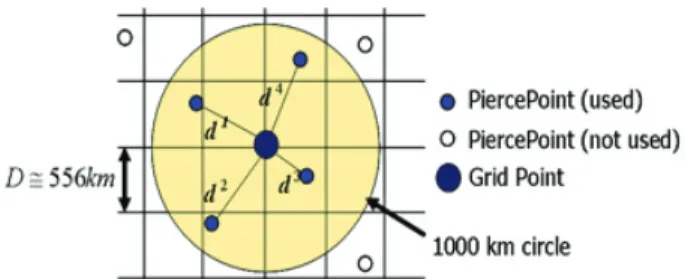
The grid model estimates and provides the predefined vertical ionospheric delay value of a grid point, and the ionospheric delay is corrected by calculating the ionospheric delay value at a specific ionospheric pierce point from the ionospheric delay value of the grid point.
For the standard grid model of WADGPS, the grid interval of 5° in the latitude and longitude directions is generally used. Fig. 2 shows the conceptual diagram for estimating the vertical ionospheric delay value of a grid point from the ionospheric delay measurements, and the ionospheric delay value of the grid point is estimated using the measurements that are within a certain radius of each grid point. The weighted interpolation is used as the estimation method, and the calculation equation is shown in Eq. (5) (Kim 2007). The ratio of ionospheric delay measurement for the Klobuchar model value is interpolated rather than simply interpolating the ionospheric delay measurement, and this is to secure the trend for the local time.
(5)
where
: Vertical ionospheric delay estimated at a grid point
: Vertical ionospheric delay estimated at a grid point using Klobuchar model
: Vertical ionospheric delay estimated at the ionospheric pierce point of a measurement using Klobuchar model
: Measured vertical ionospheric delay : Weight for each measurement
The weight for each measurement is a value that can vary depending on how it is defined by the user. In this paper, the weight was made to be inversely proportional to the distance and measurement variance. The ionospheric delay value at the ionospheric pierce point, which is to be obtained from the ionospheric delay value of the grid point, is calculated in a similar way to the above procedure.
3.2 Spherical harmonics model
The spherical harmonics refer to the basis functions which are orthogonal one another on a sphere as shown in Fig. 3. A certain data on a sphere can be expressed as a linear combination of these basis functions, and when the vertical ionospheric delay value is expressed as spherical harmonics, it is as shown in Eq. (6) (Kim 2007).
(6)
where
IV: Vertical ionospheric delay
: Magnetic latitude of an ionospheric pierce point : Local time of an ionospheric pierce point which normalized 24 hours as 2π
N, M: Maximum degree and order : Spherical harmonics coefficient : associated Legendre function
In Eq. (6), the vertical ionospheric delay value is obtained from the L1 and L2 frequency measurements, and the magnetic latitude and local time of an ionospheric pierce point are calculated from the latitude and longitude for the ionospheric pierce point of a measurement. n and m refer to degree and order, respectively. The degree determines resolution in the latitude direction, and the order
Fig. 2. Conceptual figure of grid point and pierce point.
Fig. 3. Spherical Harmonic functions.
determines resolution in the longitude direction. In other words, as the maximum degree and order values become larger, more detailed and precise expressions are possible in the latitude and longitude directions, respectively. In theory, as the maximum degree and order increase, more precise modeling is enabled, and if it is used as a post-processing model for the entire globe, the values are typically set to more than 10. However, if it is used as a model for providing the real-time correction, the maximum degree and order values need to be adjusted appropriately considering computation and the delivery of correction. The spherical harmonics coefficient is the unknown which is to be estimated. If the spherical harmonics expression for the measurement is rearranged by letting this coefficient be x, it is as shown in Eq. (7).
(7)
where
From Eq. (7), the coefficient is estimated as shown in Eq.
(8) using the least square method.
(8)
When the coefficient is obtained, the vertical ionospheric delay value at a specific ionospheric pierce point can be calculated from Eq. (6).
4. MODELING PERFORMANCE TEST 4.1 Data collection
The performance test was carried out using the measurements obtained from the NDGPS reference stations of the Ministry of Land, Transport and Maritime Affairs.
The Daejeon, Palmido, Eocheongdo, Sokcho, and Dokdo reference stations were used, and a day (July 2, 2012) was selected which has no anomalies such as ionospheric storm. The ionospheric delay measurement was obtained by filtering the data which was stored every second in the
BINary EXchange format and the data for a 24-hour period was used.
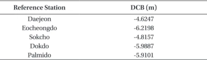
When the data from a number of reference stations are used, the DCB value should be removed which is induced by the electrical path difference between the L1 frequency signal processing circuit and the L2 signal processing circuit. Every satellite DCB value can be removed in the data processing procedure of each reference station using the Time of Group Delay value of the navigation data provided by the GPS satellite. The DCB value for each reference station is calculated by collecting the data from every reference station, and can be estimated along with the spherical harmonics coefficient by adding the reference station DCB term to the spherical harmonics expression of the ionospheric delay measurement (Kim 2007). The test was conducted in a post-processing way. As the reference station DCB value does not change greatly for a day, the DCB value was estimated by processing the data for the entire test period at a time, and the estimated DCB value was removed from every ionospheric delay measurement prior to using the measurement. Table 1 lists the estimated reference station DCB values.
Fig. 4. Position of Korea NDGPS reference stations (blue) and Grid Point (red).
Table 1. DCB of reference station.
Reference Station DCB (m)
Daejeon Eocheongdo
Sokcho Dokdo Palmido
-4.6247 -6.2198 -4.8157 -5.9887 -5.9101