Temporal Changes of Direction and Spatial Frequency Tuning in Visual Cortex Areas 17 and 18

Temporal Changes of Direction and Spatial Frequency Tuning in Visual Cortex Areas 17 and 18

Jong-Nam Kim*

Laboratory of Veterinary Neuroscience and Research Institute for Veterinary Science, College of Veterinary Medicine, Seoul National University, Seoul, Korea

Spatial frequency and direction tuning to drifting sinusoidal gratings are intrinsic properties of neurons in visual cortex neurons in areas 17 and 18. To investigate the stability of these tuning properties during visual stimulation in anesthetized cats, the temporal dynamics of spatial frequency and direction tuning were analyzed in every 0.1 sec. The responses of cortical neurons (n=109) as a function of spatial frequency as well as direction at a particular velocity for 1 second were measured and plotted as a contour plot. Five parameters from this plot were extracted: optimum response, preferred direction (direction that showed the optimum response), optimum spatial frequency (spatial frequency that showed the optimum response), direction tuning width (the difference between the highest and lowest directions to which the cell was at least half as responsive as it was to its optimum direction) and spatial frequency bandwidth (the difference between the highest and lowest frequencies to which the cell was at least half as responsive as it was to its optimum frequency). Then, this contour plot was further analyzed in every 0.1 sec to investigate whether these five parameters were changed or not during the course of stimulation. These parameters were plotted along the time (0.1 sec step) and a line of fit was found. Both spatial frequency and direction tuning properties were not changed in most of the cells. This suggests that both direction and spatial frequency tuning properties are stable during drifting sinusoidal gratings

stimulation.

Key words: Feline, temporal dynamics, electrophysiology, sinusoidal grating, visual cortex

(Received 5 January 2010; Revised version received 15 March 2010; Accepted 17 March 2010)

It has been known that most visual cortex neurons in areas 17 and 18 of anesthetized and paralyzed cats are selective along the dimension of either spatial frequency (Campbell

et al

., 1969; Maffei and Fiorentini, 1973; Tolhurst and Movshon, 1975; Movshon

., 1978; De Valois

., 1982) or direction (Campbell

., 1968) of drifting sinusoidal grating stimuli.

In the domain of spatial frequency tuning, the decrease of spatial frequency bandwidth was found (Bredfeldt and Ringach, 2002). Preferred spatial frequency was also changed (Mazer

., 2002; Nishimoto

., 2005). The preferred spatial frequency changes from low spatial frequencies to high spatial frequencies through time when stationary gratings

were flashed on for 200 msec (Frazor

., 2004) or for 20 msec (Bredfeldt and Ringach, 2002).

In the domain of orientation tuning, the narrowing of the orientation tuning bandwidth were found (Volgushev

., 1995; Ringach

., 1997; 2003) including the change of the preferred orientation (Chen

., 2005). More than forty percent of cells show a significant change in either preferred orientation or tuning width between early and late portions of the response within 150 msec (Schummers

., 2007).

On the other hand, some reports suggest that the preferred orientation (Mazer

., 2002; Nishimoto

., 2005) and tuning width were temporally stable (Celebrini

., 1993) in intracellular recordings experiments (Gillespie

., 2001) or in voltage-sensitive dyes experiments (Sharon and Grinvald, 2002).

Above mentioned experiments were done by using stationary flashed gratings for a very short duration (less than 200 msec). The question is whether there are any temporal changes in the spatial frequency selectivity and direction tuning

*Corresponding author: Jong-Nam Kim, Lab of Veterinary Neuroscience and Research Institute for Veterinary Science, College of Veterinary Medicine, Seoul National University, San 56-1, Shillim-Dong, Seoul 151-742, Korea

Tel: +82-2-880-1251

Fax: +82-2-6280-1251

E-mail: [email protected]

Materials and Methods

Animal preparation

Cortical responses were recorded in areas 17 and 18 in the cat. All experimental procedures were approved by the Seoul National University Animal Care and Use Committee.

All recordings were made from three adult cats weighing between 3 and 4 kgs (Hanlym Lab. Animal Co.). Atropine (0.05 mg) and dexamethasone (40 mg) were injected subcutaneously to reduce tracheal secretions and minimize the stress response, respectively. Cats were initially anesthetized with a mixture of Ketamine and Xylazine (15 mg/kg and 1.5 mg/kg; I.M). An endotracheal tube was inserted to allow for artificial respiration and each cat was anesthetized with 2- 3% isofluorane (0.5% in O

during the recording). The head of the animal was secured in a revised stereotaxic device (Boardtech, Korea) with the use of ear and mouth bars and clamps on the orbital rim. Then a stainless steel peg, which was implanted on the frontal bone, was secured later in the stereotaxic device. A craniotomy was made over the lateral gyrus of the left hemisphere and the dura was reflected.

After stabilization of anesthesia, the animal was immobilized with gallamine triethiodide (10 mg). Respiratory rate and volume were controlled by respiratory pump (Clare ventilator, Australia). The end-tidal CO

level and body temperature were maintained at 3.8-4.2% and 37.5

C, respectively. The infusion fluid thereafter contained gallamine triethiodide (10 mg/kg per hr), and glucose (80

g/kg/h) in Ringer solution.

The eyes were treated with 10% phenylephrine (Neodynephrine-POS, Ursa pharm.) and 0.1% atropine, and protected with a zero power contact lens. Retinal coordinates were obtained. Artificial pupils (5 mm diameter) were placed in front of the eyes. A trial lens (usually between

2 and

−

3 diopters) was placed in front of the right eye to correct the distance while the left eye was occluded.

Then the stimulus was centered in the middle of several (about three or five) cells

minimum receptive fields.

The primary purpose of this study is to measure whether there are temporal changes of spatial frequency tuning and/

or direction tuning of visual cortex neurons, on a 0.1 sec time scale, over the course of 1 sec. Therefore direction and spatial frequency tuning selectivity was measured at the same time by drifting gratings as described in the following text.

Drifting sinusoidal gratings were viewed within a square aperture (15 deg

15 deg). The spatial frequency and directional tuning properties of neurons were examined with drifting sinusoidal gratings of varying spatial frequencies, velocities and directions (Jones

., 1987; Hammond and Pomfrett, 1990; Park and Kim, 2004). The experimental design involved testing a series of ten spatial frequencies and sixteen directions at seven velocities (i.e. total number of stimuli=

1120). At a particular spatial frequency (0.05 cycle/deg) and orientation (67.5 deg), the stimulus was shown for 1 sec at a particular velocity (60, 50.8, 41.5, 32.3, 23.1, 13.9, 4.6,

4.6,

13.9,

23.1,

32.3,

41.5,

50.8 and

60.0 deg/

sec) one by one. This set was repeated at seven other orientations as well (-22.5 deg intervals). Between orientations, a blank screen was interspersed for 3 seconds. After all orientations and velocities were shown, the same sequence was repeated at nine other spatial frequencies (0.27, 0.48, 0.70, 0.92, 1.13, 1.35, 1.57, 1.78 and 2.0 cycles/deg).

Therefore, the whole set provided 1120 responses and 80 resting discharges. This test was repeated two or four times.

Electrophysiological recording

Single and/or multiple units were recorded extracellularly

from areas 17 and 18 with a Utah multielectrode array (UEA,

Bionic Technologies, Inc., USA). The UEA was implanted to

a depth of 1.5 or 1.0 mm by a high-velocity inserter (Rousche

and Normann, 1992) at the junction of the lateral and posterior

lateral gyri based on cortical landmarks provided (Tusa

al

., 1978).

Neural activity was amplified (5000

), filtered (250-7500 Hz), and digitized to the neural signals (8 bits, selectable resolution of 0.5-8

V per bit, 30000 samples per second) by a 100-channel data acquisition system (Bionic Technologies Inc., USA). At the end of a recording session, the animals were given a lethal dose of pentobarbital in excess of 100 mg/kg body weight I.V.

Data analysis

We performed a unit classification off-line by a Matlab Sorting Program v2.0 Beta (Bionic Technologies, Inc., USA).

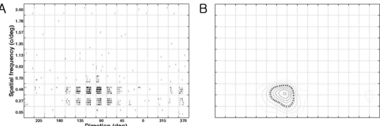
The responses of a neuron to 160 stimuli (10 spatial frequencies

×

16 directions) at the optimal velocity (during 1 second) are shown as raster plots in direction versus spatial frequency domain (Figure 1A). The horizontal axis ranges from 0 to 337.5 and represents

Direction

, while the vertical axis ranges from 0.05 to 2.0 cycle/deg and represents

Spatial Frequency

. In each small box four raster plots were shown vertically as a stimulus was repeated four times. The horizontal axis in each box represents

Time

and the first half indicates

‘

during stimulation (i.e. response) for 1 sec

and the other half is a blank period (i.e. spontaneous activity) for 1 second.

The net firing rate was calculated as the difference between the firing rates during the blank and stimulation. Mean firing rates (n=4, or n=2) were averaged for each stimulus (10

×

16 array). After adding one last column with the first column (i.e. 10

17 array), the new array was processed further by

‘

interp2 (cubic)

function that produced a contour plot with a 201

341 array. Two-dimensional tuning contour plots of

a joint direction and spatial frequency domain are shown in Figure 1B. The center of inner-most contour is the optimal response and it is located at the optimal direction (along the x-axis) and the optimal spatial frequency (along the y- axis). The contour at the 50% of the optimal response was indicated by asterisks and direction tuning width and spatial frequency bandwidth were calculated by measuring horizontal distance or vertical distance of the boundary, respectively.

The response in the null direction was calculated when it showed some. To estimate the extent of directionality, the directionality index (DI) was computed as 1 minus the ratio of the response in the null direction to the response in the preferred direction. Therefore, seven values were extracted from one contour plot. However, only five parameters excluding null direction and directionality were analyzed further in this paper.

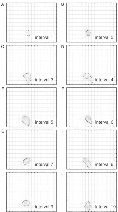
Ten contour plots (intervals 1-10) were prepared in every 0.1 sec from the beginning of the stimulation to see temporal dynamics of spatial frequency and direction tuning (Figure 2). From each contour plot, five values were calculated and plotted along the interval time (or number) and a line of best fit was found (Figure 3). The distribution of the slope of the fitted line was shown in Figure 4.

Results

Recordings were made from a total of 172 cells as a function of spatial frequency and direction. Sixty-three cells were discarded because there was a noise during recordings in an unexpected manner. This noise made it difficult to find

Figure 1.

Quantification of direction/spatial frequency tuning plot (cell number: 0709_c65_u3_v5). The stimuli were sinusoidal gratings with 10 spatial frequencies (the y-axis) in 16 directions (22.5 deg interval, the x-axis) at a particular velocity (4.6 deg/sec).

(A). Raster plots of responses of a neuron in a joint direction and spatial frequency domain. Raster plots show responses to 160

different stimuli (combinations of 10 spatial frequencies and 16 directions). (B). The contour plot in a joint direction and spatial

frequency domain. The contour at the 50 % of the maximum response, at the optimal direction (x-axis) and at the optimal spatial

frequency (y-axis), is indicated by asterisks. Therefore, five values were calculated (optimal response: 45 impulses/sec, optimal

direction: 104.6 deg, tuning width: 47.4 deg, optimal spatial frequency: 0.46 c/deg, bandwidth: 0.36 c/deg) from this contour plot

after measuring two more values including horizontal distance (i.e. tuning width) and vertical distance (i.e. bandwidth) of the

boundary.

Figure 2.

Temporal analysis of the response of the cell shown in Figure 1. The contour plot in Figure 1B was analyzed in every 100

msec, from the beginning of the stimulation to the end of stimulation, to draw 10 contour plots. Figure 2A is the contour plot at the

1st interval time (between 0 and 0.1 sec) and Figure 2J is the contour plot at the 10th interval time (between 0.9-1.0 sec). The

shapes of the boundary at the 50% of the optimal response are slightly different among them. But, it is generally a round shape

even though it shows two peaks in Figure 2D (i.e. the 4th interval time). The size of the boundary becomes bigger at the 3rd interval

and becomes similar up to the 10th interval.

optimal response by a program especially when the analysis time was short (i.e. 0.1 sec). Therefore, 109 cells were selected for further analysis. The contour plot during 1 sec is shown

in Figure 1B while 10 contour plots in each 0.1 sec are shown in Figure 2.

Figures 1B and 2 show typical 2-D selectivity maps for

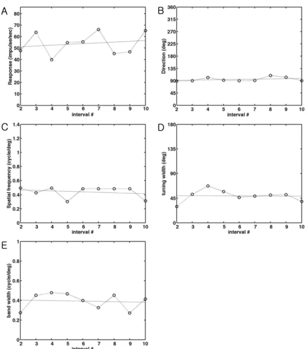
Figure 3.

The changes of parameters during stimulation. Each parameter measured in every 0.1 sec is plotted against the number

of interval time between the 2nd interval and 10th interval to quantify the change. The parameters at the 1st interval are not

included because the peak at the 1st interval is generally weak. A line of fit was found to see the increase or decrease of these

parameters during stimulation and was also drawn in the same graph. The meaning of the slope of the fitted line is the changes of

values from the 2nd interval to the 10th interval time. Positive values indicate the increase of parameter, whereas negative values

indicate the decrease of parameter. (A). The change of optimal response. The optimal response measured in each interval is

plotted as a function of time. The slope of a fitting line is 0.07 which means not much change during stimulation. (B). The change of

optimal direction. The optimal direction measured in each interval is plotted as a function of time. The slope of a fitting line is 0.93

which means 10 degree change during stimulation. (C). The change of optimal spatial frequency. The optimal spatial frequency

measured in each interval is plotted as a function of time. The slope of a fitting line is 0.007, which means 0.63 cycle/degree change

during stimulation. (D). The change of tuning width. The direction tuning width measured in each interval is plotted as a function of

time. The slope of a fitting line is -0.10, which means 1 degree change during stimulation. (E). The change of spatial frequency

bandwidth. The spatial frequency bandwidth at each interval is plotted as a function of time. The slope of a fitting line is 0.003, which

means 0.03 cycle/degree change during stimulation.

a cell obtained with drifting gratings. The data were obtained at 10 spatial frequencies and 16 directions (22.5 degree steps) of drifting sinusoidal gratings. The position of the center of inner-most contour in Figure 1B indicates that the optimal grating parameters are 104.6 degree for the direction (along the x-axis) and 0.46 c/deg for the spatial frequency (along the y-axis). The optimal response at the optimal direction and optimal spatial frequency is 45 impulses/sec while the

tuning width is 47.4 degrees and bandwidth is 0.36 c/deg.

In Figure 2, the shapes of the boundary at the 50% of the optimal response, indicated by asterisks, are slightly different among 10 interval times. But, they are generally round shapes even though it showed two peaks in the 4th interval time. The size of the 50% boundary becomes bigger from the 3rd interval and becomes similar up to 10th interval.

To quantify this change, the width (i.e. direction tuning width)

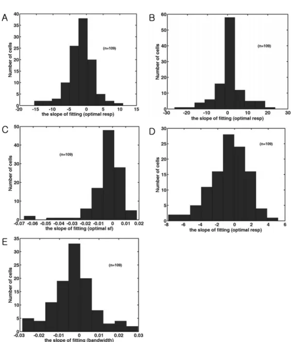
Figure 4.

The distribution of the slope of fitting line of five parameters. (A). Histogram of the slope of fitting line in the optimal

response of the time-averaged response of each cell. (B). Histogram of the slope of fitting line in the optimal direction of the time-

averaged response of each cell. (C). Histogram of the slope of fitting line in the optimal spatial frequency of the time-averaged

response of each cell. Positive numbers indicate a shift from low to high spatial frequencies, whereas negative numbers indicate a

shift from high to low spatial frequencies. (D). Histogram of the slope of fitting line in the direction tuning width of the time-averaged

response of each cell. A positive value indicates that the tuning width is increased. (E). Histogram of the spatial frequency

bandwidth of the time-averaged response of each cell.

and the height (i.e. bandwidth) of the boundary at the optimal direction and the optimal spatial frequency were calculated and plotted along the interval time (Figure 3) and found a line of fit. The values in the 1st interval were not used in Figure 3 because the response during the 1st interval was generally weak.

The meaning of the slope of the fitted line is the changes of values from the 2nd interval to the 10th interval time.

Positive values indicate the increase of parameter, whereas negative values indicate the decrease of parameter. Therefore, the value of 5 in the x–axis in Figure 4A means 45 impulses/

sec (=5

9 interval times) increase during stimulation. On the other hand, the value of 5 in the x-axis in Figure 4B means 45 degree change during stimulation. The meaning of other slopes in Figure 4 can be interpreted in the same manner.

The strength of optimal response tends to be weaker (Figure 4A). 72 cells showed a weaker response while 37 cells showed a stronger response (mean=

1.72, SD=3.92). The optimal direction (mean=0.22, SD=7.08) was not changed (Figure 4B). Tuning width (mean=

0.73, SD=2.30) in some cells was narrowed (Figure 4D).

The optimal spatial frequency (mean=

0.004, SD=0.013) was decreased slightly (Figure 4C) while the bandwidth was narrowed (mean=

0.003, SD=0.011) (Figure 4E).

Discussion

During visual stimulation with a stationary stimulus, temporal dynamics of spatial frequency and orientation tuning were tested by several scientists. While optimal orientation is not changed, optimal spatial frequency is changed and tuning width or bandwidth is generally narrowed, even though some scientists do not have the same results. These results were obtained in a short duration of stimulation, usually less than 200 msec stimulation.

In our experiment, a drifting grating was used instead of a stationary stimulus. Even though the duration was much longer (i.e. 1 sec), some narrowness of tuning width and/

or bandwidth was found in some cells. It was interesting that direction properties and spatial frequency properties were not stable during stimulation in some of the cells. This means that some suppression exists in the intercortical level as suggested in a stationary grating stimulation test (Shapley

al

., 2003; 2007; Malone and Ringach, 2008).

When a multi channel recording system is adapted as in our experiment, various parameters should be selected because neurons

optimal parameters are different among cells. This means that the experiment becomes time consuming

especially when a drifting stimulus is used as a stimulus. It takes 40 minutes in our experiment to use such a big grating (15 degree

15 degree) with various parameters (1120 stimuli) with a blank; It takes 3-4 seconds to prepare such a big stimulus in our Pentium 4 computer. More time is needed to do an experiment if a resting discharge is recorded every time before stimulation.

When a stationary stimulus is used, the stimulus duration can be decreased to 200 msec or even 40 msec. When a drifting grating is used instead, one second is used traditionally for a stimulus duration. If direction and spatial frequency tuning properties were stable during stimulation as suggested in this experiment, the next question is how long the duration of stimulation can be shorten to get reasonable tuning properties of spatial frequency and direction when drifting grating stimuli are used.

When we see a drifting grating, we instantly recognize the kind of stimulus. But, when we are stimulating neurons in an anaesthetized and paralyzed cat with a same stimulus, one neuron’s responses are very variable. The response is not always same to a certain stimulus every time. Therefore, one second of stimulation is used traditionally. However, results found in this experiment suggest that 0.1 second is enough for stimulation in some cells.

Acknowledgments

The author thanks M.A. Leem for her valuable technical assistance. This work was supported by Seoul National University.

References

Bredfeldt, C.E. and Ringach, D.L. (2002) Dynamics of spatial frequency tuning in macaque V1.

22(5), 1976- 1984.

Campbell, F.W., Cleland, B.G., Cooper, G.F. and Enroth-Cugell, C. (1968) The angular selectivity of visual cortical cells to moving gratings.

198(1), 237-250.

Campbell, F.W., Cooper, G.F. and Enroth-Cugell, C. (1969) The spatial selectivity of the visual cells of the cat.

203(1), 223-235.

Celebrini, S., Thorpe, S., Trotter, Y. and Imbert, M. (1993) Dynamics of orientation coding in area V1 of the awake primate.

10(5), 811-825.

Chen, G., Dan, Y., and Li, C.Y. (2005) Stimulation of non- classical receptive field enhances orientation selectivity in the cat.

564(1), 233-243.

De Valois, R.L., Albrecht, D.G. and Thorell, L.G. (1982) Spatial frequency selectivity of cells in macaque visual cortex.

Res.

22(5), 545-559.

Frazor, R.A., Albrecht, D.G., Geisler, W.S. and Crane, A.M.

(2004) Visual cortex neurons of monkeys and cats: temporal dynamics of the spatial frequency response function.

Neurophysiol.

91(6), 2607-2627.

Fourier domain. J. Neurophysiol. 100(1), 239-248.

Mazer, J.A., Vinje, W.E., McDermott, J., Schiller, P.H. and Gallant, J.L. (2002) Spatial frequency and orientation tuning dynamics in area V1. Proc. Natl. Acad. Sci. U S A. 99(3), 1645-1650.

Movshon, J.A., Thompson, I.D. and Tolhurst, D.J. (1978) Spatial and temporal contrast sensitivity of neurones in areas 17 and 18 of the cat's visual cortex. J. Physiol. 283(1), 101-120.

Nishimoto, S., Arai, M. and Ohzawa, I. (2005) Accuracy of subspace mapping of spatiotemporal frequency domain visual receptive fields. J. Neurophysiol. 93(6), 3524-3536.

Park, Y. and Kim, J.N. (2004) Spatial frequency and velocity tunings of neurons in areas 17 and 18 of the cat using a 100 microelectrode array. Korean J. Lab. Anim. Sci. 20(1), 26-30.

Ringach, D.L., Hawken, M.J. and Shapley, R. (1997) Dynamics of orientation tuning in macaque primary visual cortex. Nature,

visual responses in the primary visual cortex. Prog. Brain Res.

165(1), 21-32.

Sharon, D. and Grinvald, A. (2002) Dynamics and constancy in cortical spatiotemporal patterns of orientation processing.

Science 295(5554), 512-515.

Tolhurst, D.J. and Movshon, J.A. (1975) Spatial and temporal contrast sensitivity of striate cortical neurones. Nature 257(5528), 674-675.

Tusa, R.J., Palmer, L.A. and Rosenquist, A.C. (1978) The retinotopic organization of area 17 (striate cortex) in the cat.

J. Comp. Neurol. 177(2), 213-235.

Volgushev, M., Vidyasagar, T.R. and Pei, X. (1995) Dynamics of

the orientation tuning of postsynaptic potentials in the cat

visual cortex. Vis. Neurosci. 12(4), 621-628.