재료역학과 구조역학 수업을 위한 전산프로그램 개발
Development of New Computer Program for Mechanics of Materials and Structural Mechanics Courses
이 상 순*
Sang Soon Lee*
Key Words : Solid and Structural Mechanics, Mechanics of Materials, Visual C++, Visual SolidMech
ABSTRACT
The new computer program, visual SolidMech (ver 2.0), for mechanics of materials and structural mechanics has been developed using visual C++. The visual SolidMech is organized in a format similar to most standard texts on mechanics of materials and structural mechanics. This program consists of a number of menus to perform various calculations as well as a set of dedicated graphical user interfaces. Solutions to problems are given in both graphical and numerical forms. The visual SolidMech will help students develop problem-solving skills by showing them the important factors affecting various problem types, by helping them visualize the nature of internal stresses and member deformations, and by providing them an easy-to-use means of investigating a greater number of problems and variations. This new program can be utilized as a supplement to existing texts in mechanics of materials and structural mechanics.
* 한국기술교육대학교메카트로닉스공학부([email protected]) 제1저자 (First Author) : 이상순
교신저자 : 이상순 접수일자: 2011년 12월 1일 수정일자: 2011년 12월 16일 확정일자:2011년 12월 16일
Ⅰ. Introduction
Mechanics of materials and structural mechanics are the fundamental and important course in mechanical engineering, aerospace engineering, civil engineering, and architecture engineering. A thorough grounding in ideas of mechanics of materials and structural mechanics is essential to understand many topics of design and reliability analysis courses. The solutions to many problems in mechanics of materials and structural mechanics are more interesting when the tedium of excessive hand numerical computations is avoided. In addition, with the use of the computer, more thought can be given to the significance of the solution and to the effect on the solution of changing input parameters in the problem. Greater insight into the solution can be also provided by making use of graphics to plot results in the solution.
The computer program for solid and structural mechanics course has been developed by several investigators. Lardner and Archer(1994) developed the computer program for mechanics of materials course, MECHMAT.This program is written in BASIC and the source code is available. Solutions to problems are given primarily in numerical forms. Nash(1998) developed the FORTRAN(or BASIC) programs for stress analysis. These programs require some knowledge for FORTRAN (or BASIC) program and give the solutions to problems in numerical forms. Turcotte and Wilson(1998) and Golnaraghi et al.(1999) developed the computer program to solve mechanics of materials problems, using MATLAB.
Numerical computation and visualization of results can be easily performed. These programs, however, require some information for MATLAB environment. The purpose of this study is to develop the computer program as a supplemental tool for the mechanics of materials and structural mechanics course using visual C++. A unique feature of this computer program, visual SolidMech(ver. 2.0), is that it is suitable for
engineering students at the undergraduate level and for students who are totally new to the computer programming. Geometrical or graphical illustrations are included in the program wherever they are appropriate. In this computer program, computer graphics are used to exhibit clearly the solution. As a consequence, design changes can be explored more fully, and the programs can be used effectively with the text to introduce notions of a design approach.
Ⅱ. Visual SolidMech (ver 2.0)
The visual SolidMech(ver 2.0) is organized in a format similar to most standard texts on mechanics of materials and structural mechanics.
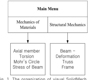
This program consists of a number of menus to perform various calculations as well as a set of dedicated graphical user interfaces. The program covers axial load, torsion, Mohr’s circle, bending of beam, and elementary structural members(see Fig.1). The detailed procedure for data input and visualization of results is given in next NUMERICAL EXAMPLES.
Main Menu
Mechanics of
Materials Structural Mechanics
Axial member Torsion Mohr’s Circle Stress of Beam
Beam - Deformation
Truss Frame
Fig. 1. The organization of visual SolidMech.
ⅡI. THEORETICAL BACKGROUND
The theoretical background on the visual SolidMech(ver. 2.0) is briefly covered in this chapter.
1. Axial Load Problems
A member under axial loading undergoes deflection along its longitudinal axes. There are two classes of problems: statically determinate and statically indeterminate. In the first case, all reaction and applied axial forces in the member are solvable using equilibrium equation. A member under axial loading is statically indeterminate if the unknown forces are not attainable using the equilibrium equations alone. In that case, one must supplement the equilibrium equations with additional equations pertaining to the displacements of the member.
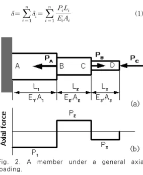
If a bar is subjected to a number of axial loads at different points along the bar, or if the bar consists of parts having different cross-sectional areas or of parts composed of different materials (Fig. 2a), then the change in length of the various parts of bar can be added algebraically to give the total change in length of the complete bar as follows:
(1)
Fig. 2. A member under a general axial loading.
where and are the cross-sectional area and the length of segment , respectively, and is Young’s modulus of segment . The force is the internal force in segment of the bar and is
usually different than the forces applied at the ends of the segment. These forces must be calculated from equilibrium of the segment and are often shown on axial force diagram such as Fig.
2b. The normal stress in segment is given as follows:
(2)
2. Torsion Problems
A circular shaft under torsion undergoes a rotation. There are two classes of problems:
statically determinate and statically indeterminate.
In the first case, all reaction moments in the circular shaft are solvable using equilibrium equation. A shaft under torsional loading is statically indeterminate if the unknown moments can not be solved using the equilibrium equations alone. In that case, one must supplement the equilibrium equations with additional equations pertaining to the rotation of the shaft.
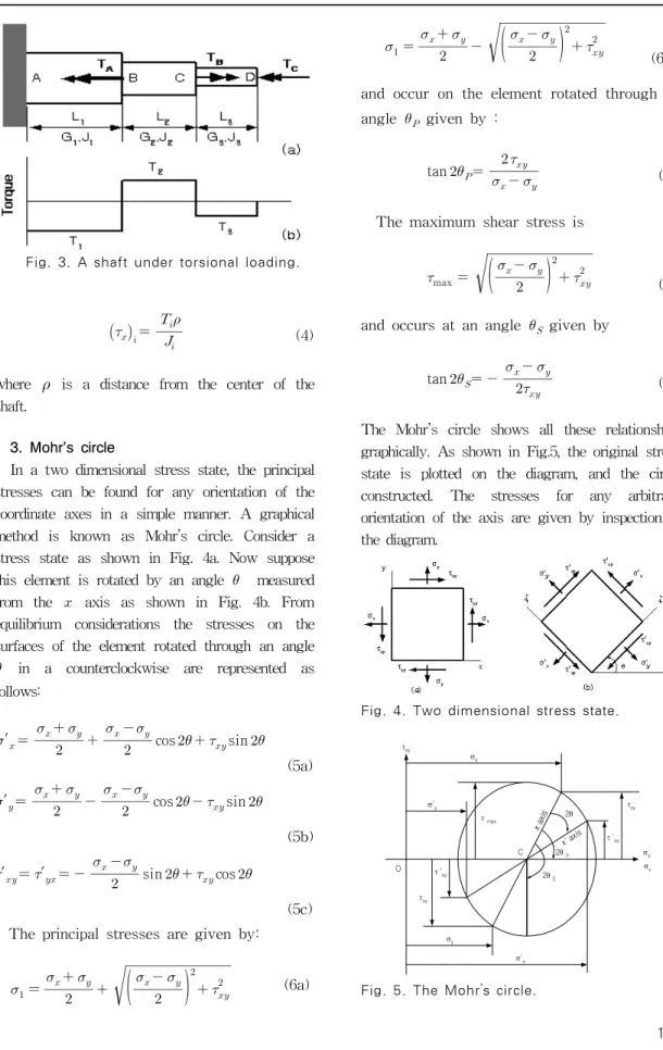
If a shaft is subjected to a number of torques at different points along the shaft, or if the shaft consists of parts having different cross-sectional areas or of parts composed of different materials (Fig. 3a), then the angle of twist of the various parts of shaft can be added algebraically to give the total amount of twist of the complete shaft as follows:
(3)
where and are the polar second moment of area and the length of segment , respectively, and is the shear modulus of segment . The torque is the internal torque in segment of the shaft and is usually different than the torques applied at the ends of the segment. These torques must be calculated from equilibrium of the segment and are often shown on torque diagram such as Fig. 3b.
The shear stress in segment is given as follows:
′
cos sin
Fig. 3. A shaft under torsional loading.
(4)
where is a distance from the center of the shaft.
3. Mohr’s circle
In a two dimensional stress state, the principal stresses can be found for any orientation of the coordinate axes in a simple manner. A graphical method is known as Mohr’s circle. Consider a stress state as shown in Fig. 4a. Now suppose this element is rotated by an angle measured from the axis as shown in Fig. 4b. From equilibrium considerations the stresses on the surfaces of the element rotated through an angle
in a counterclockwise are represented as follows:
(5a)
′
cos sin
(5b)
′ ′
sin cos
(5c) The principal stresses are given by:
(6a)
(6b) and occur on the element rotated through an angle given by :
tan
(7)
The maximum shear stress is
max
(8) and occurs at an angle given by
tan
(9)
The Mohr’s circle shows all these relationships graphically. As shown in Fig.5, the original stress state is plotted on the diagram, and the circle constructed. The stresses for any arbitrary orientation of the axis are given by inspection of the diagram.
Fig. 4. Two dimensional stress state.
τxy
σx σy
2θ S 2θP
2θ σx
σ'x σ'y
τmax x axis
x' axis τxy
τ 'xy C
O τ 'xy τxy
σy
Fig. 5. The Mohr’s circle.
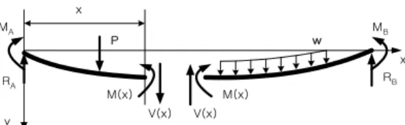
4. Bending of Beam
In engineering, beams are treated by an approximate elastic theory. Referring to Fig.6, is measured from the left end of the beam. is measured positively downward and represents the deflection of the beam. Moments may be applied at the ends as shown. Positive moments tend to bend the beam concave upward as shown. The beam may be cut at any point, and the necessary shear force and bending moment
determined in order to hold the beam in equilibrium, as shown in Fig.7.
The equation for deflection is given as follows:
(10)
where is the moment in the beam, is the cross-sectional area moment of inertia about the neutral axis on the cross section, and is Young’s modulus. Additional useful equations for small deflection are :
(11a)
and
(11b)
where is the loading per unit length of the beam. Therefore,
12a)
(12b)
M M
x
y
L y x
Fig. 6. The simple beam.
MA MB
x
y
x
RA RB
w P
M(x) M(x)
V(x) V(x)
Fig. 7. Shear forces and bending moments in a beam.
For a simple beam as shown in Fig. 7, the stresses consist of bending normal stresses acting on the cross section, and shear stresses acting on a cross section. For a symmetric cross section the bending stress is given as follows:
(13)
where is the bending moment at the value of
where the stress is computed, is the distance from the neutral axis, and is the cross-sectional area moment of inertia about the neutral axis on the cross section.
The shear stress for simple cross sections is given by:
(14)
Here is the shear on the surface, is the first moment of the part of the cross section defined by a line through the point where the stress is determined and the outer extremity of the section.
This first moment is taken about the neutral axis.
is the width of the section at the point where the shear stress is calculated (Fig. 8).
neutral axis z
y1 c
b Line of interest
to find τxy
Fig. 8. Shear stress in a simple beam.
IV. Numerical Examples
In order to demonstrate the convenience and the effectiveness of the visual SolidMech program, 3 examples are tested.
Example 1. A steel bar is loaded by 3 forces as shown in Fig.9. The total length of the bar is 12 m. Calculate the change in length of the bar and the axial stresses developed in the bar.
3m 3m 2m 2m 2m
E1, d1 E2, d2
E3, d3 E4, d4 E5, d5
P1 P2 P3
,
,
Fig. 9. Steel Bar subjected to 3 forces.
The following steps demonstrate how to solve this problem using visual SolidMech.
Enter the visual SolidMech program by clicking the SolidMech. The main menu shown in Fig.10 appears. Next click the 'mecahnics of materials' button. Then, the sub menu shown in Fig.11 will appear on the screen.
Fig. 10. Main Menu
Fig. 11. Sub menu
Next click the 'Axially loaded member' button.
Then, the Fig.12 window will appear on the screen. Click the 'Uniform member' button in Fig.12. Then, the window shown in Fig. 13 appears.
Fig. 12. Problem type.
Fig. 13. Cross-sectional areas.
We now enter the geometric data(Fig.14) and the modulus of elasticity(Fig.15) related to steel bar of Fig.9. Click the next button of Fig.12. Then, the Fig.16 window will appear. We enter the load
data. The result is shown in Fig.17.
Fig. 14. Input window for the geometric data.
Fig. 15. Input window for the material property.
Fig. 16. Input window for the load data.
Fig. 17. Stress and displacement of an axially loaded member.
EXAMPLE 2. A continuous beam of a H-type cross section is supported and loaded as shown in Fig. 18. Determine the maximum tensile and compressive stresses in the beam. Also, determine the maximum deflection.
2m 4m 6m
7m 8m
10 kN/m 10 kN/m 10 kN
10 kNm
Fig. 18. Continuous beam.
The shear force diagram and the bending moment diagram are shown in Fig.18. The stress and deflection of the beam is shown in Fig. 19.
Fig. 19. Shear force and bending moment diagrams.
Fig. 20. Stress and deflection of beam.
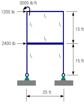
EXAMPLE 3. Consider the frame shown in Fig 21. The frame is made of steel, with
× . The cross-sectional area is
and the second moment of areas for the members are and . We are interested in determing the deformation of the frame under the given loads.
I2 I1
I1 I1
I1 I1
15 ft
15 ft
25 ft 2400 lb
1200 lb
3000 lb.ft
Fig. 21. The steel frame.
The result using the visual SolidMech is shown in Fig.22.
Fig. 22. Deformation of the frame.
V. Conclusions
The new computer program, visual SolidMech(ver. 2.0), for mechanics of materials and structural mechanics courses has been developed using visual C++. This program consists of a number of menus to perform various
calculations as well as a set of dedicated graphical user interfaces. These graphical user interfaces are very intuitive and provide a learning environment where students can focus on understanding and solving various problems rather than typing cumbersome expressions and checking numerical errors. Solutions to problems are given in both graphical and numerical forms.
The visual SolidMech will help students develop problem-solving skills by showing them the important factors affecting various problem types, by helping them visualize the nature of internal stresses and member deformations, and by providing them an easy-to-use means of investigating a greater number of problems and variations. An emphasis is placed on using the visual SolidMech as a learning aid rather than a comprehensive industry-class package. It is concluded that the visual SolidMech can be utilized as a supplement to existing texts in mechanics of materials and structural mechanics.
참 고 문 헌
[1] Lardner, T.J. and Archer, R.R. (1994), Mechanics of Solids, McGraw-Hill, Inc.
[2] Nash, W. (1998), Strength of Materials (schaum’s outlines), 4th ed., McGraw-Hill International Editions.
[3] Turcotte, L.H. and Wilson, H.B. (1998), Computer Applications in Mechanics of Materials Using MATLAB, Prentice Hall.
[4] Golnaraghi, M.F., Boulahbal, D., and Leask, R.L. (1999), Solving Solid Mechanics Problems with MATLAB 5, Prentice Hall.
이 상 순 (Sang Soon Lee) 정회원
KAIST 기계공학과와 미국
UCLA에서 각각 기계공학 석사와 박사학위를 취득하였고, 현재는
한국기술교육대학교 메카트로닉
스 공학부에서 교수로 재직하고 있다.
<관심분야> 전산고체역학, 동적시스템 해석, 신뢰성 공학