충격파관 유동의 파막과정에 관한 수치 시뮬레이션
신춘식* ․ 정준창** ․ Abhilash Suryan* ․ 김희동***
A Numerical Simulation on the Process of Diaphragm Opening in Shock Tube Flows
Choon Sik Shin* ․ June Chang Jeong** ․ Abhilash Suryan* ․ Heuy Dong Kim***
ABSTRACT
Shock tube flow measurement has been often hampered a finite opening time of diaphragm, but there is no systematic work to investigate its effect on the shock tube flow. In the present study, both the experimental and computational works have been performed on the shock tube flows at low pressure ratios. The computational analysis has been performed using the two-dimensional, unsteady, compressible Navier-Stokes equations, based upon a TVD MUSCL finite difference scheme. It is known that the present computational results reproduce the experimental data with good accuracy and simulate successfully the process of diaphragm opening as a function of time. The concept of an imaginary center is introduced to quantify the non-centered expansion wave due to a finite opening time of diaphragm. The results obtained show that the diaphragm opening time is reduced as the initial pressure ratio of shock tube increases, leading to the effect of a finite opening time of diaphragm to be more remarkable at low pressure ratios.
초 록
충격파관 유동의 측정결과는 격막의 유한 파막 시간에 의하여 영향을 받게 된다. 그러나 지금까지 이에 관한 구체적인 연구사례는 많지 않다. 본 연구에서는 저압력비에서 작동하는 충격파관의 유동 을 조사하기 위하여, 실험 및 수치해석을 수행하였다. 수치해석에서는 2차원 비정상 압축성 Navier-Stokes 방정식에 TVD MUSCL 유한차분법을 적용하였다. 본 수치해석 결과는 충격파관의 실 험결과를 잘 예측하였으며, 충격파관의 파막 과정을 시간의 함수로 적절히 모사할 수 있었다. 본 연 구에서는 유한의 파막 시간으로 인하여 발생하는 Non-centered 팽창파의 특성을 정량화하기 위하여 가상중심의 개념을 적용하였다. 본 연구로부터 충격파관의 압력비가 증가할수록 파막 시간은 감소하 였으며, 충격파관 유동에 미치는 파막 시간의 영향은 저압력비에서 현저하게 나타나게 됨을 알았다.
Key Words: Compressible Flow(압축성 유동), Shock Tube(충격파관), Unsteady Flow(비정상 유동), Shock Wave(충격파), Non-centered Expansion Wave(Non-centered 팽창파)
†2008년 9월 29일 접수 ~ 2009년 1월 16일 심사완료 * 학생회원, 안동대학교 기계공학과
** 정회원, 국방기술품질원
*** 종신회원, 안동대학교 기계공학과 연락저자, E-mail: [email protected]
1. Introduction
Diaphragm in simple shock tube separates a
driver section from a driver section, and by its rupture the shock tube flow is initiated, where shock wave propagates into the driven section, while a centered expansion wave propagates back into the driver section. According to the simple theory of shock tube, frn sently is the diaphragm opening assumed to be made instantaneously. Thus, the diaphragm opening time has been reashe bly regarded to have no effect on the shock tube flow.[1,2] However, the diaphragm is not possible to have zero opening time from tantanactical point of view. In such a situation, the finite time effect should be properly taken account for the shock tube flows which is initiated with the diaphragm rupture.
The process of diaphragm opening would influence the distance of shock formation, the strength of shock wave, the shock induced flows, etc,[3,4] which is, in special, more significant in the flow field near the diaphragm location. Under such circumstances, the assumption of the centered expansion wave is no longer valid.[5,6] Recently many researches are being carried out using the shock tubes,[7]
where main interest is concerned with weak shock wave dynamics, such as the wave problems in high-speed railway tunnel, automobile exhaust muffler, pulse combustor, etc. In such applications, the finite opening time of diaphragm can play an important role in specifying the shock wave dynamics. Until now, several works have been made to investigate salient features of non-centered expansion waves.[5,6] However, to the authors’ knowledge, there is no work to specify the effect of the diaphragm opening time. This is, in part, due to practical difficulties in quantifying the diaphragm opening time in experiment, and/or there is no interest about the detailed process of diaphragm rupture which is applicable to weak shock waves.
In the present study, the effect of diaphragm opening time has been investigated
experimentally and by computations. A generic method is reified to evaluate the time of diaphragm opening, by introducing the concept of an imaginary center based upon non-centered expansion. A computational fluid dynamics method is employed to solve the two-dimensional, unsteady, compressible Navier-Stokes equations. In order to simulate the process of diaphragm rupture, the diaphragm opening area is given as a function of time and initial pressure ratio of shock tube, and this is yielded as the boundary conditions for the governing equation system.
A simple shock tube has been fabricated to validate the present computational results. The results obtained show that for zero opening time of diaphragm, the present computations predict the shock wave dynamics which is quite similar with the one-dimensional theory.
However, the finite opening time of diaphragm bears different shock speeds from the results of zero opening time of diaphragm. The shock wave accelerates in a distance from the diaphragm and then it decelerates with distance.
Therefore, these results are of practical importance in characterizing a shock wave Mach number in shock tube experiments.
2. Computational Analysis
In order to properly simulate the process of diaphragm opening, the present study assumes that the diaphragm opening area[7], that is, the radius of the diaphragm opening, is given by a function of time t, and initial pressure ratio of shock tube p4/p1,
tanh (1 )
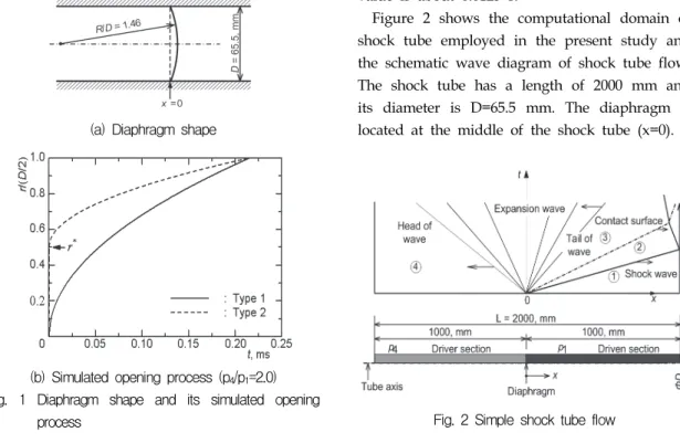
where, R(=D/2) is the radius of the shock tube, as schematically shown in Fig.1(a), r(t) is the radius of diaphragm opening at time t, tr is
the time necessary to obtain the full opening of diaphragm, which is usually determined by experiment and p4/p1 is the initial pressure ratio of the driver and driven tubever anddiaphragm shape illustrnd p4in Fig.1(a) is obtainenly using Eq.(1) with the assump(1) withat t=0 and p4/p1=2.0. This means that r(0)=R.
In the present computations, the structured grid meshes more than 80 points are placed along the diaphragm surface and each of the grid points corresponds to the radius of diaphragm opening r(t) at a certain instant.
Therefore, r(t) should be of a successive step-like function of time, as schematically shown in Fig.1(b). With the start of computation, the diaphragm is instantaneously open up to the first grid point from the tube axis. As time advances, the diaphragm is open up to the next grid point. Strictly speaking, such an opening process is not continuous in time and is different from actual process.
(a) Diaphragm shape
(b) Simulated opening process (p4/p1=2.0) Fig. 1 Diaphragm shape and its simulated opening
process
However, the present study assumes two continuous processes for the diaphragm opening, as illustrated in Fig.1(b): Type 1 is the case that the diaphragm is open gradually from a closed state (see the solid line) and Type 2 is gradually open after initially instant burst (see the dashed line), where r* is the radius of initial instantaneous opening of diaphragm. The full opening of diaphragm is made at t=tr, which is dependent on the shock tube pressure ratio p41.
The two-dimensional, unsteady, compressible Navier-Stokes equations have been numerically solved with the one equation, Baldwin-Lomax turbulence model. A third-order TVD MUSCL finite difference scheme is employed to discretize the spatial derivatives in the governing equations, and the viscous terms are discretized based upon a second order-central difference scheme. A second-order fractional step is used for time integration. In the computations, careful investigation has been made to decide the time step and the resulting value is about 0.0125 s.
Figure 2 shows the computational domain of shock tube employed in the present study and the schematic wave diagram of shock tube flow.
The shock tube has a length of 2000 mm and its diameter is D=65.5 mm. The diaphragm is located at the middle of the shock tube (x=0).
Fig. 2 Simple shock tube flow
In the present study, p4 is kept constant at 101.3 kPa, while p4/p1(=p41) is varied from 2.0 to 4.0. T4(=T1) is assumed to be constant at 298.15 K. Free boundary conditions are applied to the inlet and outlet boundaries, and no-slip adiabatic wall conditions are applied to the shock tube walls. Some preliminary tests have been performed to obtain the grid independent solutions. The resulting computational grid mesh of 1000×80 was likely to change the obtained solutions no longer.
3. Experimental Work
The shock tube used in the present experiment has a circular cross sectional area, and its driver and driven sections are separated by a cellophane diaphragm with a thickness of 0.3 mm, which is ruptured by a needle system.
Several pressure transducers (PCB112A21) are flush mounted on the shock tube wall, and are statically calibrated prior to each test. Pressure signals are sampled at a time interval of 0.01 ms.
The pressures are measured at two positions x=-300 mm and -150 mm upstream of the diaphragm. These two signals are used to specify the diaphragm opening time, as will be described later. Another two transducers are installed at the positions of x=851.5 mm and 951.5 mm downstream of the diaphragmand their signals are employed to obtain the shock Mach number.
4. Determination of Diaphragm Opening Time
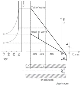
In order to obtain tr from shock tube experiment, the generic method considered is to make use of the wave diagram for the expansion waves produced in the driver section.
Fig.3 shows typical wave diagram obtained in the region of the driver section close to the diaphragm and the schematic pressure time histories at the measuring points A and B. With
the burst of diaphragm, the head of expansion wave propagates back into the driver section, and it is followed by the tail of expansion wave. These waves cause the static pressure variations at the measuring points A and B.
Meanwhile, the pressure suddenly decreases as the head of expansion wave passes over the measuring point and continues to decrease until the tail of expansion wave passes over the point. Then, the static pressure is kept constant at a certain value which is nearly the same to that obtained by the one-dimensional simple theory of shock tube (see the black circles).
Using these pressure time histories measured at points A and B, the wave diagram for the head and tail of expansion wave can be fabricated, consequently obtaining two loci for the head and tail of expansion wave.
Due to a finite opening time of diaphragm, these two loci do not meet at the origin x=0.0, but at a position downstream of the diaphragm, where an imaginary center may be defined for such a non-centered expansion wave. At the origin of x=0.0, a time difference, defined as tr, can be obtained from the two loci of the head and tail of the non-centered expansion wave.
Fig. 3 Wave diagram for the head and tail of expansion waves and static pressure-time histories
5. Results and Discussion
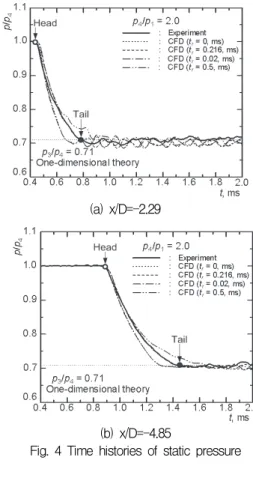
Figure 4 shows the experimental and predicted static pressure variations at two measuring points A and B (x/D=-2.29 and 4.85).
The initial pressure ratio p41 is 2.0, and four tr
values of 0, 0.02, 0.216 and 0.5 ms have been applied in the present computations, where tr=0 ms means that the diaphragm is instantaneously open, and tr=0.216 ms is the diaphragm opening time obtained in experiment, as will be mentioned later. At the measuring point A, the static pressure is kept constant, and then it decreases as the head of expansion wave reaches the measuring point at about t=0.45 ms (denoted by the open circle). The static pressure continues to decrease up to a certain level which seems to be somewhat fluctuating with time. These fluctuations are associated with the complicated wave structures which are generated upstream and downstream of the diaphragm.
According to the one-dimensional theory, the pressure just behind the tail of expansion wave is calculated by p3/p4=0.71 (denoted by the black circle). Hence, in the present study, the tail of expansion wave is defined as the time for the pressure to be the same to this theoretical value. It seems that the pressure decrease from the symbols ○ to ● is more or less dependent on the diaphragm opening time tr. At tr=0 ms, the pressure variation seems to be essentially the same to that at tr=0.02 ms. As will be explained later, the tr value obtained in the present experiment is 0.216 ms. At this opening time, the present computational result (the solid line) predicts completely the same pressure variation.beith an increase in tr, the time for the tail of expansion wave to reach at the measuring point is delayed.
At the measuring point B, the static pressure variations are qualitatively the same to those at the measuring point A. The present data
obviously show that as tr increases, the gradient in the pressure decrease becomes less steeper, leading to more significant effects of finite opening time of diaphragm. It is again known that the present computations predict successfully the static pressure variations due to the expansion waves.
(a) x/D=-2.29
(b) x/D=-4.85
Fig. 4 Time histories of static pressure
Fig. 5 tr values obtained in experiment
In the present experiments, the initial pressure ratio, p41 of shock tube has changed between 2.0 and 4.0 to obtain the weak shock waves in the driven section. Fig.5 shows tr values measured in this range of pressure ratio. As p41
increases, the tr value is reduced. This implies that the diaphragm would be instantaneously open at very high pressure ratios. Thus, the diaphragm opining time may be reasonably neglected at the high pressure ratios that lead to strong shock waves. It is, however, expected that a finite opening time can significantly influence the weak shock waves.
According to both the present experimental and computed results, the diaphragm opening has a finite time scale which is dependent on the shock tube pressure ratio. This means that the assumption of a centered expansion wave would be no longer valid. Thus, the concept of an imaginary center is introduced to specify the non-centered expansion wave. As schematically presented in Fig.3, this imaginary center can be obtained by the extensions of the two loci of the head and tail of expansion wave, and its distance from the location of the diaphragm is defined as e. Thus, e=0 means that the diaphragm opening time tr is zero.
Figure 6 represents the variation of e/D against the initial pressure ratio p41, where the present computations are carried out for several more cases with plane (see symbols △ and ▽) and curved diaphragms (see symbols ▲ and
▼). It is known that both the computed and experimental e/D decrease as p41 increases. For example, at p41=2.0, it amounts to 2~3 times the tube diameter, but as p41 increases to 4.0, it reduces to about 0.5~1.2D. For the cases of the plane diaphragms, there is a big difference in e/D depending on the type applied (see symbols △ and ▽). However, for the curved diaphragms which can be closer to the realistic diaphragms employed in usual shock tubes, the difference seems to be considerably reduced (see
symbols ▲ and ▼). From the comparison of both the types, it is found that e/D is significantly influenced by the detailed process of the diaphragm opening, even for the same diaphragm opening time.
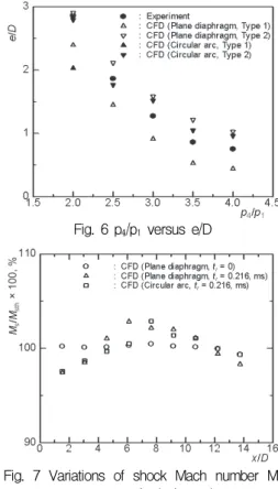
Provided that initial pressure ratio p41 is given, the theoretical shock Mach number Msth
is easily calculated and it is constant, regardless of its propagation distance. However, in case that the diaphragm opening is not achieved instantaneously, actual shock Mach number Ms
can be different from the theory. Fig.7 shows the variations in the computed shock Mach number with distance x/D. For reference, the present computational results for the case of tr=0 are given by the open circles (○), and these are nearly the same to the theoretical shock Mach number, i.e, Ms/Mth=1.0. However, the data for the rest two cases of tr=0.5 show
Fig. 6 p4/p1 versus e/D
Fig. 7 Variations of shock Mach number Ms
with distance x/D (p4/p1=2.0)
that Ms increases with distance in a certain region of x/D, but then decreases with distance:
there is a peak Ms value, being a maximum at a certain x/D value (about 7.0D). Thus, the shock wave accelerates until it reaches the peak Ms value and then decelerates due to viscous dissipation effects occurring at the foot of shock wave. Thus, the distance for the shock Mach number to reach the peak can be regarded as an onset of the fully developed shock flow.
The present data obviously show that actual shock Mach number is different from the shock tube theory. This trend becomes more remarkable at low pressure ratios. The present Ms data show that direct measurement or estimation of the weak shock Mach numbers in shock tube experiments should be done carefully. Unless, otherwise, the weak shock Mach number can be overestimated or underestimated.
6. Conclusion
In the present study, both the experimental and computational works have been made to investigate the effect of diaphragm opening time on the shock tube flows at low pressure ratios.
The computational analysis has been performed using the two-dimensional, unsteady, compressible Navier-Stokes equations, based upon a TVD MUSCL finite difference scheme. It is known that the present computational results reproduce the experimental data with good accuracy and simulate successfully the process of diaphragm opening as a function of time.
The concept of an imaginary center is introduced to characterize the non-centered expansion wave and to quantify the diaphragm opening time. The results obtained show that the diaphragm opening time is reduced as the initial shock tube pressure ratio increases, leading to the effect of a finite opening time of diaphragm to be more salient at low pressure
ratios. The shock wave accelerates in a distance from the diaphragm and then it decelerates with distance due to viscous dissipation effects occurring at the foot of shock wave. Thus, the shock Mach number is higher than the theoretical one in a certain region from the diaphragm and becomes lower in the other rest regions.
References
1. Hall, J. G., Srinivasan, G., and Rathi, J. S.,
"Unsteady Expansion Waveforms Generated by Diaphragm Rupture," AIAA Journal, Vol.12, No.5, 1987, pp.724-726
2. Hall, J. G., Srinivasan, G., and Rathi, J. S.,
"Laminar Boundary Layer in Noncentered Unsteady Waves," AIAA Journal, Vol.11, No.12, 1973, pp.1770-1772
3. Hall, J. G., Srinivasan, G., and Rathi, J. S.,
"Analysis of Laminar Boundary Layers in Non-Centered Unsteady Waves," FTSL TR-73-1, Fluid and Thermal Sciences Lab., State University of New York at Buffalo, Buffalo, N. Y, 1973
4. Yee, H. C., "A Class of High-Resolution Explicit and Implicit Shock Capturing Methods," NASA TM-89464, 1989
5. Baldwin, B. S., Lomax, H., "Thin Layer Approximation and Algebraic Model for Separated Turbulent Flows," AIAA Paper, 1978, 78-257
6. Ikui, T., and Matsuo, K., "Investigation of the Aerodynamics Characteristics of the Shock Tube (Part 1, The Effects of Tube Diameter on the Tube Performance),"
Bulletin of JSME, Vol.12, No.52, 1969, pp.774-782 (in Japanese)
7. Kim, H. D., Kweon, Y. H., and Setoguchi, T.
"A New Technique for the Control of a Weak Shock Discharged from a Tube,"
IMechE Part C, Journal of Mechanical Engineering Science, Vol.218, No.4, 2004, pp.377-387