Article Information
Manuscript Received November 25, 2019, Revised January 30, 2020, Accepted September 11, 2020, Published online June 30, 2021 The authors are with KEPCO Research Institute, Korea Electric Power Corporation, 105 Munji-ro Yuseong-gu, Daejeon 34056, Republic of Korea.
Correspondence Author: In-sung Jeon ([email protected])
This paper is an open access article licensed under a Creative Commons Attribution-NonCommercial-NoDerivatives 4.0 International Public License.
To view a copy of this license, visit http://creativecommons.org/licenses/by-nc-nd/4.0
This paper, color print of one or more figures in this paper, and/or supplementary information are available at http://journal.kepco.co.kr.
Environmental change due to construction of large offshore wind farm has been a debate for a long time in Korea. There are various data acquired on hydrodynamics around this area before and during construction of offshore wind farm but no data during operation could be made due to delayed schedule. In this study, environmental change such as bathymetry change and scouring was forecasted using MIKE, numerical hydrodynamics model, and its results were validated using the observation data before and during construction.
Keywords: Numerical Model, Offshore Wind Farm, MIKE21/3
I. Background and Necessity
ince the government’s announcement of renewable energy policy 3020 to increase the percentage of renewable energy production by 20% by 2030, the research on large scale offshore wind farm has been carried out. In 2017, demonstration site of 60 MW size was commenced and as of now, only the underwater cable construction is remaining before commercial operation in November 2020. There were so much opposition to the construction of offshore wind farm due to environmental effect it might cause around the area. There had been many research projects carried out to study the environmental impact of offshore wind farm and environmental monitoring project is one of them. In environmental monitoring, remote sensing devices such as multibeam echosounder, x-band radar, 3D scanner, wave gliders were used to monitor marine hydrodynamics like waves, current, wind, bathymetry, and so on to assess the impact of offshore wind farm around the area. But due to the opposition, commercial operation was delayed and data during operation are not available for study of actual impact on the area.
In this study, therefore, environmental impact of offshore wind farm, specifically morphology change and scour, were simulated using MIKE and their impacts were analyzed. For validation of the model, observation data before and during construction were used.
II. Methodology
For the numerical model formulation, observation data is crucial in defining current status and for the validation. Korea Electric Power Corporation (KEPCO) carried out government project to develop the remote environmental monitoring system
that uses sound pulses and other types of waves to gather ocean data such as current, wave, bathymetry, and so on. These data were first analyzed and later, will be used in the numerical model for simulation of future phenomenon.
S
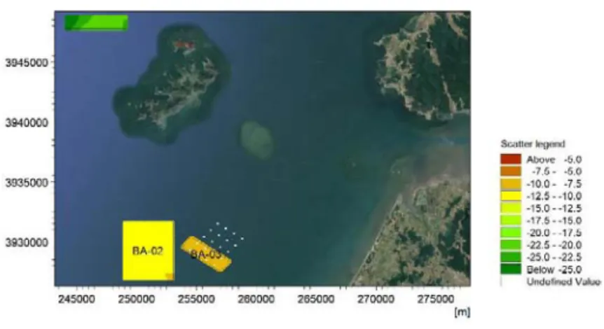
Fig. 1. Location of bathymetry data.
TABLE 1 Bathymetry Data No Data
name
Horizontal reference
Vertical
reference Resolution Time 1 BA-01 UTM-52N LAT 10 m 2014.11~2015.03 2 BA-02 UTM-52N LAT 10 m 2014.11~2015.03 3 BA-03 UTM-52N LAT 10 m 2017.12~2018.02
2018.05 2018.10~2018.11
146
A. Analysis of Data
Bathymetry data in three different areas around South West offshore wind farm were measured for various periods before and during construction as in Fig. 1 and TABLE 1.
These bathymetry data are used in the formulation of local model around South West offshore wind farm as nested depth data.
For wind speed and direction, offshore metmast data from HeMOSU1 was used. The period for the data is from 1st march 2008 to 22nd July 2014 and time step is 3 hours as in Fig. 2.
Water level and currents are also measured for various points around the area for different periods. They range from far offshore to coastal area. The location and the periods are listed in Fig. 3 and TABLE 2.
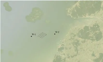
Wave data is also measured for various periods at two points which location and detailed information listed in Fig. 4 and TABLE 3.
Apart from the above listed data, there are various other data used in this study like simulation significant wave data for extreme wave analysis, typhoon data, and so on.
B. Hydrodynamic Modelling
For MIKE21, Hydrodynamic Model (HD) is based on DHI’s Flow Model (FM) module which is 2D free-surface depth-integrated flow model that is based on 2D incompressible Reynolds-averaged Navier-Stokes equations subject to the assumptions of Boussinesq and of hydrostatic pressure. HD model includes both astronomical tide and surge forced by the meteorological data and will give results in water level, current speed and direction.
There will be two different model set up for accurate forecast, one being regional HD model and another, local HD model. Regional HD model includes the area of Bohai bay to South East part of Korean Fig. 2. Wind rose plot of HeMOSU1.
Fig. 3. Location of current and water level measurement stations used.
TABLE 2
Water Level and Current Data
Station Latitude Longitude Depth Period Type of data T-1 126.25417 35.47500 -10.8 2014.11.13~2014.12.12
2015.02.10~2015.03.11 2015.04.23~2015.05.22 2015.07.29~2015.08.27 2016.02.04~2016.03.04
Water level T-2 126.39222 35.48833 -5.2
PC-1 126.25417 35.47500 -10.8 2014.11.13~2014.12.12 2015.04.23~2015.05.22
2015.07.29~2015.08.27 Current PC-2 126.25194 35.42194 -9.4 2014.11.13~2014.12.12
2015.04.23~2015.05.22
2016.02.04~2016.03.04 Current PC-3 126.16806 35.46361 -11.5 2015.04.23~2015.05.22 Current
PC-4 126.39222 35.48833 -5.2
2014.11.13~2014.12.12 2015.04.23~2015.05.22 2015.07.29~2015.08.27 2016.02.04~2016.03.04
Current
PC-5 126.42500 35.55056 -5.5 2018.09.~2018.10. Current PC-6 126.39361 35.42639 -4.0 2018.04.~2018.05.
2018.09.~2018.10. Current PC-7 126.39250 35.48806 -5.2 2017.12.~2018.01.
2018.04.~2018.05.
2018.09.~2018.10. Current
Fig. 4. Location of wave measurement stations.
TABLE 3 Wave Data
Station Latitude Longitude Depth Period Type of data W-1 126.2541667 35.475 -10.8 2014.11.13~2014.12.12
2015.04.23~2015.05.22 2015.07.29~2015.08.27 Wave
W-2 126.3922222 35.4883 -5.2
2014.11.13~2014.12.12 2015.04.23~2015.05.22 2015.07.29~2015.08.27 2016.02.04~2016.03.04
Wave
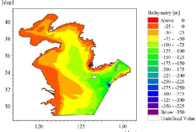
Fig. 5. Regional model domain and bathymetry.
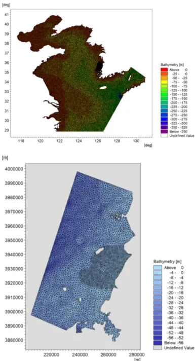
Fig. 6. Local model domain and bathymetry.
TABLE 5 Sensitivity Test Cases
Case Manning number Wind Friction Eddy Viscosity
1 35 2 m/s 0.001225
10 m/s 0.004525 0.45
2 40 2 m/s 0.001225
10 m/s 0.004525 0.45
3 45 2 m/s 0.001225
10 m/s 0.004525 0.45
4 Varying 2 m/s 0.001225
10 m/s 0.004525 0.45
5 Varying 2 m/s 0.001225
10 m/s 0.002538 0.45
6 Varying 2 m/s 0.001225
10 m/s 0.004525 0.28
Fig. 7. Time series comparison of water level.
Fig. 8. Time series comparison of current.
peninsula. Model domain and bathymetry of the regional model is shown in Fig. 5.
For three open boundaries, boundary conditions of regional model are got from global ocean tide model DTU10. MIKE uses triangular flexible mesh and the grid size can vary from complicated terrain to simpler ones and mesh resolution is about 5,000 m. Other parameters of regional HD model are listed in TABLE 4.
To achieve high quality results in simulation of environmental impact, high-resolution local HD model using observation data for bathymetry and other data is used with nesting techniques. Local model domain and bathymetry is shown in Fig. 6.
For local model, there are parameters which has to go through sensitivity test as a calibration of the model. Usually in the ocean, some of the parameters vary from area to area and hence empirical values are generally used for simulation but in this case, since we do not have enough experimental data, sensitivity tests are carried out for the best simulation of the model. The cases for sensitivity test are shown in TABLE 5.
The results were compared with the observation data to find out which case simulates better. With various tests, case 5 was found to simulate the result with minimum differences. For manning coefficient, 40m1/3/s was used for water depth less than 25 m, and 47m1/3/s otherwise and other values of wind friction and Eddy viscosity are shown in the above table. Comparison of model and observation results are shown in Fig. 7 through Fig. 9.
C. Wave Modelling
Wave is an important parameter when dealing with ocean environment since wave induced shear stress is a key factor for sediment suspension and morphology change. Also, wave induced currents from typhoons and high waves will result in bathymetry change and scour as well. In this study, wind forcing from CFSR (Climate Forecast System Reanalysis) data will be used to get 50 years return-period significant wave height. This will be used several times to simulate extreme events for morphology and scour change.
Wave model used in this study is spectral wave (SW) model which is based on an unstructured, cell-centered finite volume method and uses unstructured mesh. The model is able to simulate the growth, decay and transformation of wind-generated waves and also swells in offshore and coastal areas. The SW model also uses regional domain and local domain mesh which was used in the simulation of HD model. Domain and mesh for spectral wave models are shown in Fig. 11.
Calibration test is carried out for the wave model. Parameters include bottom friction, Energy transfer including triad-wave Fig. 9. Scatter plot comparison for current speed
Fig. 10. Wind rose comparison for wind
Fig. 11. Domain and mesh for regional (top) and local (bottom) SW model.
interaction, white capping, and so on and they are listed in TABLE 6.
In MIKE21, SW allows the use of a coupled, uncoupled or spatially-varying specifications to estimate surface roughness and in this study, spatially-varying approach was used and it is shown in Fig. 12.
It is quite important for wind-generated waves such as typhoons and high waves during winter, to define limit on wind drag coefficient. The effect of wind drag is shown in Fig. 13.
After the calibration test, final model set up of local SW model is shown at TABLE 7.
D. Scour
South West offshore wind farm was constructed in relatively shallow water (depth of 10-30 m) and wave induced currents cause the movable sea floor sediments interact with the turbine foundation resulting in scour hole development. This is caused by change of the flow pattern which can be described as horseshoe and lee-wake vortices. Horseshoe vortex is formed in front of the pile which is caused by rotation of incoming flow which then undergoes a three-dimensional separation that increases the shear stress in Fig. 13. Time series of significant waveheight at HEMOSU1 during the
Tembin, CAP value of 0.065 (top), and 0.06 (bottom).
1.5.b Ddis
(white-capping distribution) 0.337 1.6 Air-Sea interaction Uncoupled
(Nearshore) Short fetch
1.7.a Gamma
(depth-induced breaking) 0.9 Extremes (shallow)
1.7.b Gamma
(depth-induced breaking) 1.0
TABLE 7
Summary of Local SW Model Set Up
Setting Value
Mesh resolution varying
Basic equations Fully spectral in-stationary Time step (adaptive) 0.01-3,600 s
Water level HD local model
Current speed Not included.
Energy Transfer Triad-wave interaction included Wind forcing CFSR, typhoon parameter varying Air/water density
ratio Varying in time and domain, calculated from CFSR Wave breaking Included, Specified Gamma, γ=1, α= 1 Bottom friction Nikuradse, kn = 0.005 m
White-capping Formulation: Cdis =2.106 (offshore) Cdis=1.87(nearshore), DELTAdis =0.337 Boundary
conditions 2D spectra varying in time and along lines from Yellow Sea Wave Model Output
specifications 1-hourly, integrated wave parameters at every mesh element
Fig. 14. Scour mechanism around cylindrical pile.
front of the pile up to 5 times or larger than the undisturbed bed shear stress. For lee-wake vortex which is caused by the rotation in the boundary layer over the surface of the pile, the shear layer from side edges of the pile roll up to form this vortex behind the pile and it can reach up to 4 to 10 times undisturbed ones. It is shown in Fig.
14.
The scour calculation for MIKE model assumes that the seabed near the pile always develops towards an equilibrium scour depth determined by the actual environmental condition, in which case we have the observation data, and scour depth and width at each time step are calculated based on bed shear stress.
The mean bed shear stress τmean is a function of the bed shear stress for current, τc and the bed shear stress for wave, τw and a coefficient, Y which depends on the choice of bed shear stress metho d and the internal angle between waves and current.
𝜏𝑚𝑒𝑎𝑛= 𝑌(𝜏𝑐+ 𝜏𝑤) (1)
The bed shear stress for current only, τc is related to the depth- averaged current, V, through the drag coeffient, CD, by
𝜏𝑐= 𝜌𝐶𝐷𝑉2 (2)
where
𝐶𝐷= [ 0.4 1 + ln(𝑧0⁄ )ℎ ]
2
(3)
where h is the water depth, 𝑧0= 𝑘𝑠⁄30 and 𝑘𝑠= 2.5 × 𝑑50. The bed shear stress for waves only, τw, is expressed by
𝜏𝑤= 0.5𝜌𝑓𝑤𝑈𝑤2 (4)
where fw is the friction factor for the wave and Uw is the velocity at the seabed.
The friction factor wave fw is calculated as
𝑓𝑤= 1.39 (𝐴 𝑧0)
−0.52
(5)
where 𝐴 = 𝑈𝑤𝑇 (2𝜌)⁄ .
The velocity Uw is found by
𝑈𝑤= 𝜋𝐻𝑠
𝑇𝑝sinh(𝑘ℎ) (6)
The design parameters used for jacket structure for the model is given as in TABLE 8.
III. Results
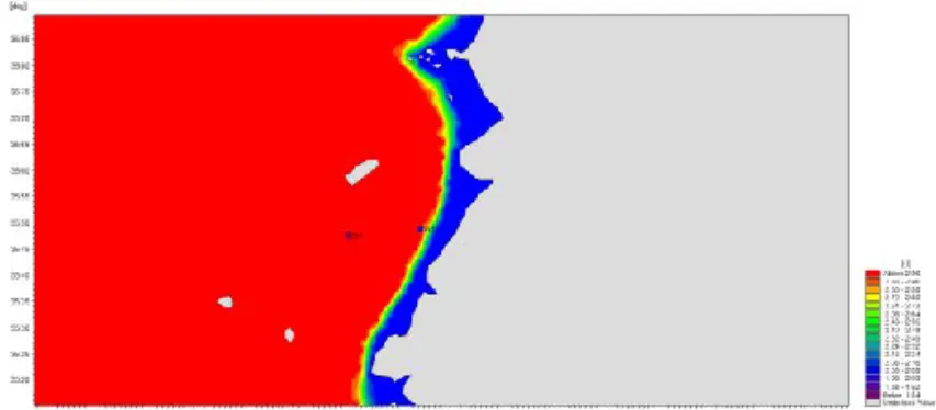
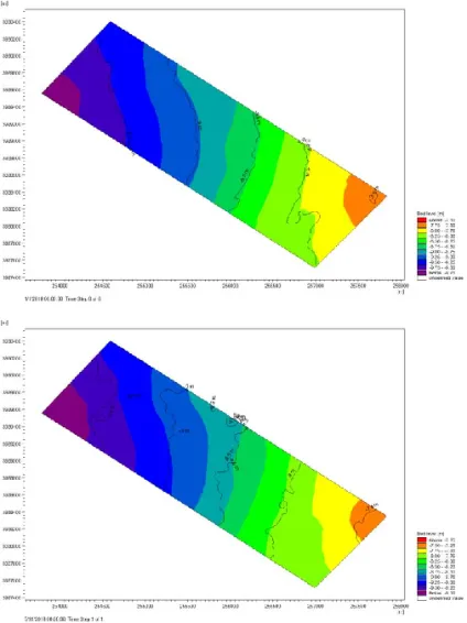
A. Bathymetry Change
To simulate the partial discharge inside a gas-insulated transformer, an experiment was performed by applying IEC 60270.
First, within a 2L-sized partial discharge cell, 99.999% pure SF6 gas was injected with the gauge pressure, one barMorphological calculations were made using MIKE21 and the simulation period is 5 months (January 2018-May 2018) and the simulation results were compared with the observation data.
The solid line in Fig. 15 shows the observation data and colored area shows the model results. The sedimentation occurs during winter monsoon and it can be seen in the above figure that isobath of different water depth moves towards west. but due to computational time limit and coarse mesh, the isobath does not fit so well after simulation for 5 months. Still, we can see that the model represents the tendency of accretion quite well.
The impact of wind turbines was also simulated and the results without wind turbines and result with turbines in place were compared to see the overall impact on seabed as in Fig. 16.
24-hour simulation of 50-year return period wave condition was used and the results show that water depth increase of 10-20 cm per year on average but this is obviously due to monsoon. The overall bed thickness is about 0.02 cm near the wind turbine which is considered to be negligible.
B. Scour
The equilibrium scour depth was found out to be 1.9 m from the simulation by mud transport model from MIKE and time scale for equilibrium scour depth was tested using different current-alone cases as in Fig. 17.
Fig. 15. Modeling results in 201801 (up) and at 201805 (bottom).
TABLE 8
Design Parameters for Scour Simulation
ID Diameters
(m) Water Depth
(m) Spacing
(m) Grain size (mm)
NO.16 (Jacket) 1.115 -11.4 5.25 0.061
It was assumed that for current-alone case, current was applied continuously to reach the equilibrium scour depth and time taken was sought. It was shown that for current under 0.4 m/s, 2.1 days were taken to reach the equilibrium scour depth and for 0.6 m/s, 0.4 day, 0.8 m/s 0.1 day, and for 1 m/s, only 0.9 hours were needed.
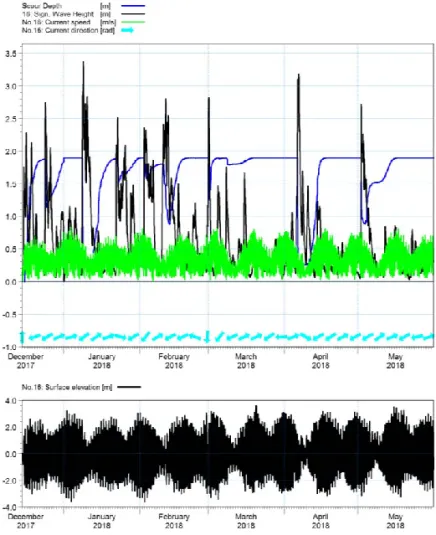
With real data from observation, simulation was made for period from December 2017 - May 2018 and the scour development of No. 16 jacket foundation were compared.
It is shown in Fig.18 that current increases scouring depth but the waves cause deposition and this pattern repeats. With relatively high waves above 1.5 m cause deposition but for current, the rate at which scour depth increases is proportional to current speed.
IV. Conclusion
Observation before and during construction of South West offshore wind farm were made and data were used but since the operation of offshore wind farm was not made, its’ environmental change was simulated using numerical software, MIKE21. Results show about 0.02 cm change of bathymetry by offshore wind turbines which can be negligible. For scour, about 1.9m of equilibrium scour depth was simulated and this result show good agreement with
observation data which was about 1.9 m to 2 m. It was also shown that current increases scour depth and during high waves, deposition occurs. More studies should be made and observation data must be acquired during operation of offshore wind farm to confirm the results of numerical simulation.
Acknowledgment
This work was supported by the New & Renewable Energy of the Korea Institute of Energy Technology Evaluation and Planning (KETEP) grant funded by Ministry of Trade, Industry and Energy, Korea (No. 20203030020080, Environmental impact analysis on the offshore wind farm and database system development).
References
[1] Bidlot, J., Jansen, P., Abdalla, S., “A Revised Formulation of Ocean Wave Dissipation and Its Model Impact,” p. 509, 2007.
[2] Chao, Y. Y., Alves, J. H., Tolman, H. L, “An operational system for predicting hurricane-generated wind waves in the North Atlantic Ocean,” Weather Forecasting 20, pp. 652-671, 2005.
[3] Davis, R. S., “Equation for the determination of the density of moist air,” Metrologia 29(1), pp. 67-70, 1992
[4] DHI, MIKE 21, Spectral Wave Module, Scientific Documentation, Hørsholm, 2019.
[5] Janssen, P. A., “Quasi-linear theory of wind generation applied to wave forecasting,” Journal of Physical Oceanography 21, pp. 1631-1642, Fig. 17. Time scale of scour in current alone case.
Fig. 18. Scour development under wave and current conditions.
1991.
[6] Powell, M. D., “Reduced drag coefficient for high wind speeds in tropical cyclones,” Nature 422, pp. 279-283, 2003.
[7] Whitehouse, R.J.S, “Scour at Marine Structures,” Thomas Telford, London, 1998.
[8] Det Norske Veritas, “Design of Offshore Wind Turbine Structures,”
Offshore Standard DNV-OS-J101, September, p. 142, 2011.
[9] Sumer, B.M., Christiansen, N., Fredsøe, J., “Time scale of scour around a vertical pile,” Proc. 2nd Int. Offshore and Polar Engng. Conf., ISOPE, San Francisco, USA, vol. 3, pp. 308-315, 1992.
[10] Sumer, B.M., Fredsøe, J., Christiansen, N., “Scour around a vertical pile
in waves,” J. Waterway, Port, Coastal, and Ocean Engng. ASCE, vol. 118, no. 1, pp. 15-31, 1992.
[11] Breusers, H.N.C, Nicollet, G., Shen, H.W., “Local scour around cylindrical piers,” J. of Hydraulic Res., IAHR, vol.15, no.3, pp. 211-252, 1977.
[12] Audkivi, A. J., “Loose boundary hydraulics.” Pergamum Press, London, UK, 1998.
[13] B. Mutlu Sumer, Jorgen Fredsoe, “The Mechanics of Scour in the Marine Environment,” Advanced Series on Ocean Engineering-Volume 17, World Scientific Publishing Co. Pte. Ltd, 2002.