Economic analysis of a 22.9 kV HTS power cable and conventional AC power cable for an offshore wind farm connections

(1)

Vol.20, No.4, (2018), pp.60~64 https://doi.org/10.9714/psac.2018.20.4.060

```

1. INTRODUCTION

The application of wind energy and especially offshore wind energy is a keystone in the policy of several countries for large-scale use of renewable energy. The realization and the grid connection of offshore wind farms are receiving much attention [1].

As high temperature superconducting (HTS) power cables have some merits over conventional cables, several demonstration projects on the HTS cable system are presently under way around the world [2]. All HTS cables have a much higher power density than copper-based cables at similar voltage levels. Moreover, because they are actively cooled and thermally independent of the surrounding environment, they can fit into much more compact installations than conventional copper cables. In addition, HTS cables exhibit much lower resistive losses than conventional copper or aluminum conductors [3].

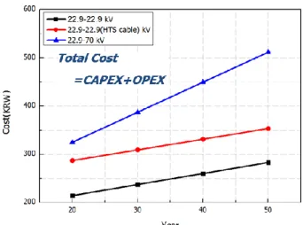
We analyzed and compared the economic feasibility of the offshore wind farm using the HTS power cable and the AC power cable. The HTS power cable used the 22.9 kV superconducting cable of LS cable&system. The economics of cable were analyzed by calculating capital expenditure (CAPEX) and operating expense (OPEX).

This paper compares three cases: 1) 22.9 kV AC power inter-array and export cables of the offshore wind farm 2) 22.9 kV AC power inter-array cables of the offshore wind

farm and 22.9 kV HTS power 22.9 kV AC power inter-array cables of the offshore wind farm and 22.9 kV HTS power export cable of the offshore wind farm to the coast and 3) 22.9 kV AC power inter-array cables of the offshore wind farm and 70 kV AC power export cable of the offshore wind farm to the coast.

For all the case studies, the case 2 is more expensive than the case 1, because of higher HTS power cable cost and cheaper than the case 3. These results can be used to economic analysis of the HTS power cable for the offshore wind farm.

2. CONFIGURATIONS OF THE OFFSHORE WIND FARM

2.1. Cable Model of the Offshore Wind Farm

The offshore wind farm submarine cable can be divided into two types of inter-array cables and export transmission cables as shown in Fig. 1.

Fig. 1. Configuration of the offshore wind farm.

Economic analysis of a 22.9 kV HTS power cable and conventional AC power cable for an offshore wind farm connections

Ga-Eun Jung, Minh-Chau Dinh, Hae-Jin Sung, Minwon Park

^*

, and In-Keun Yu Changwon National University, Changwon, Korea

(Received 30 November 2018; revised or reviewed 23 December 2018; accepted 24 December 2018)

Abstract

As the offshore wind farms increase, interest in the efficient power system configuration of submarine cables is increasing.

Currently, transmission system of the offshore wind farm uses almost AC system. High temperature superconducting (HTS) power cable of the high capacity has long been considered as an enabling technology for power transmission. The HTS cable is a feasible way to increase the transmission capacity of electric power and to provide a substantial reduction in transmission losses and a resultant effect of low CO2 emission. The HTS cable reduces its size and laying sectional area in comparison with a conventional XLPE or OF cable. This is an advantage to reduce its construction cost. In this paper, we discuss the economic feasibility of the 22.9 kV HTS power cable and the conventional AC power cables for an offshore wind farm connections. The 22.9 kV HTS power cable cost for the offshore wind farm connections was calculated based on the capital expenditure and operating expense. The economic feasibility of the HTS power cable and the AC power cables were compared for the offshore wind farm connections. In the case of the offshore wind farm with a capacity of 100 MW and a distance of 3 km to the coast, cost of the 22.9 kV HTS power cable for the offshore wind farm connections was higher than 22.9 kV AC power cable and lower than 70 kV AC power transmission cable.

Keywords: AC cable, economic analysis, offshore wind farm, superconducting cable

* Corresponding author: [email protected]

(2)

The offshore wind farm is connected to 20 wind turbines of 5 MW and the total capacity of the offshore wind farm is 100 MW. The export cable was selected as 3 km. The inter-array cables were fixed with the 22.9 kV AC power cable. Economic analysis was performed with three cases of export cable.

2.2. Three Cases of the Offshore Wind Farm

The export cable of case 1 is the 22.9 kV AC power cable and case 2 is the 22.9 kV HTS power cable and case 3 is the 70 kV AC power cable. Fig. 2-4 show three cases including the HTS power cable.

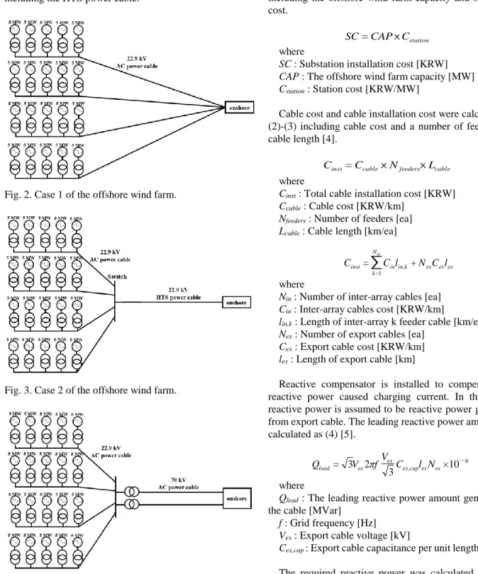
Fig. 2. Case 1 of the offshore wind farm.

Fig. 3. Case 2 of the offshore wind farm.

Fig. 4. Case 3 of the offshore wind farm.

3. COST MODELLING OF THE OFFSHORE WIND FARM

3.1. The CAPEX of the Offshore Wind Farm

The CAPEX is the money a company spends to buy, maintain, or improve its fixed assets. The CAPEX of the offshore wind farm covered substation installation cost, cable cost, cable installation cost and reactive compensator cost. The CAPEX of the offshore wind farm using HTS power cable is added cooling system installation cost.

Substation installation cost was calculated as (1) including the offshore wind farm capacity and substation cost.

station

C CAP

SC = ⅹ (1) where

SC : Substation installation cost [KRW]

CAP : The offshore wind farm capacity [MW]

C

station

: Station cost [KRW/MW]

Cable cost and cable installation cost were calculated as (2)-(3) including cable cost and a number of feeders and cable length [4].

cable feeders cable

inst

C N L

C = ⅹ ⅹ (2)

where

C

inst

: Total cable installation cost [KRW]

C

cable

: Cable cost [KRW/km]

N

feeders

: Number of feeders [ea]

L

cable

: Cable length [km/ea]

∑

^Nⁱⁿ

k

ex ex ex k in in

inst

C l N C l

C

1

=

,

+

= (3) where

N

in

: Number of inter-array cables [ea]

C

in

: Inter-array cables cost [KRW/km]

l

in,k

: Length of inter-array k feeder cable [km/ea]

N

ex

: Number of export cables [ea]

C

ex

: Export cable cost [KRW/km]

l

ex

: Length of export cable [km]

Reactive compensator is installed to compensate for reactive power caused charging current. In this paper, reactive power is assumed to be reactive power generated from export cable. The leading reactive power amount was calculated as (4) [5].

6

,

× 10

2 3 3

=

_ex ^ex _ex_cap_ex _ex ^ㅡ

lead

V C l N

π f V

Q (4)

where

Q

lead

: The leading reactive power amount generated in the cable [MVar]

f : Grid frequency [Hz]

V

ex

: Export cable voltage [kV]

C

ex,cap

: Export cable capacitance per unit length [μF/km]

The required reactive power was calculated as (5), a

reactor is installed at both ends of the cable, and half of the

(3)

required reactive power is divided between reactor and STATCOM. The installation cost of the reactive power compensator is calculated as (6) [5].

θ P

Q

_req

=

_{OW P}

tan (5)

) 2 +

( +

=

_reactor _lead _reactor _STATCOM ^req ^ex

Q

N Q C

C Q C

C (6)

where

Q

req

: The required reactive power [Mvar]

P

OWP

: Capacity of the offshore wind farm [MW]

θ : Power factor angle at 0.95 power factor [deg]

C

Q

: Total installation cost of reactive power compensator [KRW]

C

STATCOM

: STATCOM installation cost [KRW/MVar]

C

reactor

: Reactor installation cost [KRW/MVar]

The cooling system installation cost was calculated to economic analysis of the HTS power cable for the offshore wind farm (7).

cryo inst cryo

inst

C C N

Ct = ( + ) × (7) where

Ct

inst

: The total cooling system installation cost [KRW]

C

cryo

: The cryocooler cost [KRW/ea]

C

inst

: Cooling system installation cost [KRW/ea]

N

cryo

: The number of cryocoolers [ea]

3.2. The OPEX of the offshore Wind Farm

The OPEX is an ongoing cost for running a product, business, or system. The OPEX of the offshore wind farm covered substation loss cost, cable loss cost, operation and maintenance (O&M) cost. The OPEX of the offshore wind farm using HTS power cable is added cooling system loss cost and cooling system O&M cost with excepted cable loss cost.

Substation loss cost was calculated as (8) including active power, loss factor, transmission time and electricity price. The loss factor was selected as 0.8% and transmission time was selected as 6000 hours [6].

E loss

sub

P lf Tt C

C

_,

= × × × (8) where

C

sub,loss

: Substation loss cost [KRW]

P : Active power [MW]

lf : loss factor

Tt : transmission time [hrs]

C

E

: Energy generation cost per kWh [KRW/kWh]

Cable loss cost was calculated as (9)-(12) including power loss equation [4].

∑

^Nⁱⁿ

k

k in in in

k avg E

loss

in

R l

pf V C P

C

1

=

, , 2

5

,

)

( 3 3

× 10

× 8760

×

=

^ㅡ

(9)

ex ex ex ex

ex AVG E

loss

ex

R l N

pf V

N C P

C

_, ⁵

)

²

3 ( / 3

× 10

× 8760

×

=

^ㅡ

(10)

k Feeder k

avg

CF P

P

_,

= ×

_,

(11)

OW P

AVG

CF P

P = × (12) where

C

in,loss

: Inter-array cable annual loss cost [KRW]

C

ex,loss

: Export cable annual loss cost [KRW]

P

avg,k

: Average power of k feeder [MW]

P

AVG

: Average power of the offshore wind farm [MW]

V

in

: Voltage level of inter-array cable [kV]

V

ex

: Voltage level of export cable [kV]

pf : Power factor

R

in

: Resistance per length of inter-array cable [Ω/km]

R

ex

: Resistance per length of export cable [Ω/km]

CF : Capacity factor [%]

P

Feeder,k

: Total capacity of k feeder wind turbines [MW]

O&M cost was calculated as (13) including annual fault rate [4].

∑

^Nⁱⁿ

k

ex ex ex k in in repair t

m

C λ l λ l N

C

1

= ,

.

= ( + ) (13) where

C

m.t

: O&M cost of the inter-array and export cable cost [KRW]

λ

in

: Annual fault rate of the inter-array cable [times/year·km]

λ

ex

: Annual fault rate of the export cable [times/year·km]

C

repair

: Repair cost of cable at one time [KRW/times]

The cooling system loss cost was defined 20% of the submarine cable loss cost to economic analysis of the HTS power cable for the offshore wind farm.

The O&M cost of the cooling system for the offshore wind farm was calculated as (14).

cooling inst, cooling

OM

1% C

C

_,

= × (14) where

C

OM,cooling

: O&M cost of the cooling system [KRW]

C

inst,cooling

: The cooling system installation cost [KRW]

3.3. Parameters of the 22.9 kV HTS Power Cable

The HTS power cable used 22.9 kV LS cable&system data as shown in table I. The capacity of 22.9 kV HTS power cable is 120 MVA. Therefore, a 100MW offshore wind farm can be transmitted with one superconducting cable. 70kV AC cable can transmit with two cables because 70kV AC cable capacity is smaller than 100 MW.

TABLE

I

22.9

K

V HTS P

OWER

C

ABLE OF

LS C

ABLE

& S

YSTEM

.

Parameters Value Unit

Cable capacity 120 MVA

Short circuit capability 40 kA /0.5s Cross section of stabilizer 260 mm

²

Cross section of the HTS conductor 34 mm

²

Insulation thickness 4.6 mm

Cross section of the HTS shield 27.7 mm

²

Cable resistance 0.0049 μΩ/km

Cable capacitance 0.26 mF/km

(4)

The cable terminations install at both ends of the cable to install the HTS power cable. Superconducting cables can not exceed 1 km in current technology. Therefore, connecting a superconducting cable using a joint box is necessary to create a long transmission line. The HTS power cable installation cost parameters including the cable terminations and the joint boxes are shown in table II.

3.4. Parameters of the AC Power Cable and Offshore Wind Farm

The AC power cable and offshore wind farm parameters are shown in table III-V. Reference of the energy generation unit price is KEPCO industry power cost.

TABLE

II

T

HE

H

TS

P

OWER

C

ABLE

I

NSTALLATION

C

OST

.

Parameters Value Unit

HTS power cable price 4,090,000,000 KRW/km

Superconducting wire price

20,000 KRW/m

Required superconducting wires

600,000,000 KRW/km

Number of cables

175 ea

Number of joints 5 ea

Joint box price 200,000,000 KRW

Number of terminals 2 ea

Termination price 550,000,000 KRW

Cost of installation cooling system 2,000,000,000 KRW/ea Cost of cooling system 3,500,000,000 KRW/ea

TABLE

III

22.9

K

V AC P

OWER

C

ABLE

C

OST

.

Parameters Value Unit

Cable price 54,000,000 KRW/km

Cable installation cost 481,000,000 KRW/km

AC resistance 0.0766 Ω/km

Fault rate 0.0069 times/year·km

Capacitance 0.29 μF/ km

TABLE

IV

70

K

V AC P

OWER

C

ABLE

C

OST

.

Parameters Value Unit

Cable price 631,000,000 KRW/km

Cable installation cost 609,000,000 KRW/km

AC resistance 0.0631 Ω/km

Fault rate 0.00795 times/year·km

Capacitance 0.2 μF/ km

Cable repair cost 7.08 KRW/ times

TABLE

V

P

ARAMETERS OF THE

O

FFSHORE

W

IND

F

ARM

.

Parameters Value Unit

Capacity of the offshore wind

farm 100 MW

Capacity of the wind turbine 5 MW

Number of wind turbines 20 ea

Power factor 0.95

Grid frequency 60 Hz

Capacity factor 30 %

Distance between wind turbines

3.5*rotor diameter

(60 m) km

Minimum distance from wind

turbine to substation 0.5 km

STATCOM price 100,000,000 KRW/Mvar

Shunt reactor price 15,000,000 KRW/Mvar Energy generation unit price 104.43 KRW/kWh

4. RESULTS AND DISCUSSIONS

Total cost of three cases were calculated based on the equations of the CAPEX and the OPEX. The calculation results are shown in table VI-VIII. The case 2 using the 22.9 kV HTS power export cable had the lowest OPEX cost, including loss and maintenance cost. On the other hand, the cable was the most expensive. If the transmission length is long, the economic efficiency of the offshore wind farm using the superconducting cable will decrease due to the price of the superconducting cable as well as the cooling system.

The total cost calculation results are shown in Fig. 5. In the case of the offshore wind farm with a capacity of 100 MW and a distance of 3 km to the coast, case 1 was the most economical of the three cases.

TABLE

VI

C

ALCULATION

R

ESULTS OF THE

C

ASE

1. Parameters Value Unit

Cable price 937,000,000 KRW

Cable installation cost 8,350,000,000 KRW Reactive compensator price 7,572,000,000 KRW

Cable loss cost 144,000,000 KRW

Capacitance 85,000,000 KRW

Total cost 17,088,000,000 KRW

TABLE

VII

C

ALCULATION

R

ESULTS OF THE

C

ASE

2. Parameters Value Unit

Switch installation cost 30,400,000 KRW

Cable price 12,560,000,000 KRW

Cable installation cost 4,310,000,000 KRW Reactive compensator price 1,890,000,000 KRW

Cooling system

installation cost 5,500,000,000 KRW

Cable loss cost 125,000,000 KRW

O&M cost 96,000,000 KRW

Total cost 24,511,000,000 KRW

TABLE

VIII

C

ALCULATION

R

ESULTS OF THE

C

ASE

3. Parameters Value Unit

Substation installation cost 5,911,000,000 KRW

Cable price 4,075,000,000 KRW

Cable installation cost 6,232,000,000 KRW Reactive compensator price 3,814,000,000 KRW Substation loss cost 501,000,000 KRW

Cable loss cost 62,000,000 KRW

Capacitance 60,000,000 KRW

Total cost 20,655,000,000 KRW

(5)

Fig. 5. Calculation results of the three cases.

5. CONCLUSION

This paper analyzed and compared the economic feasibility of the offshore wind farm using the HTS power cable and the conventional AC power cables for the offshore wind farm. Economic analysis of the HTS power cable and the AC power cable were performed by calculating the CAPEX and OPEX. The HTS power cable had lower OPEX cost than the AC power cable. However, The HTS power cable cost is much more expensive than AC power cable cost. The price of superconducting cables and cooling systems will influence the economics of offshore wind farms. These results will be effectively utilized to analyze economic of the HTS power cable for the offshore wind farm.

ACKNOWLEDGMENT

This work was supported by the New & Renewable Energy of the Korea Institute of Energy Technology Evaluation and Planning (KETEP) grant funded by the Korea government Ministry of Knowledge Economy (No.

20183010025270).

This work was supported by the New & Renewable Energy of the Korea Institute of Energy Technology Evaluation and Planning (KETEP) grant funded by the Korea government Ministry of Knowledge Economy (No.

20183010025280).

REFERENCES

[1] Paola Bresesti, Wil L. Kling, Ralph L. Hendriks, Riccardo Vailati,

"HVDC Connection of Offshore Wind Farms to the Transmission System," IEEE Transactions on Energy Conversion, vol. 22, Issue.

1, Mar. 2007.

[2] S.H.Sohn “The Results of Installation and Preliminary Test of 22.9 kV, 50 MVA, 100 m Class HTS Power Cable System at KEPCO,”

IEEE TRANSACTIONS ON APPLIED SUPERCONDUCTIVITY, vol. 17, No. 2, Jun. 2007.

[3] J. F. Maguire, " Progress and Status of a 2G HTS Power Cable to Be Installed in the Long Island Power Authority (LIPA) Grid," IEEE TRANSACTIONS ON APPLIED SUPERCONDUCTIVITY, vol.

21, No. 3, Jun. 2011.

[4] Jong-Nam Won, "A Study on Siting on HVAC Offshore Substation for Wind Power Plant using Submarine Cable Cost Model," KIEE, vol. 62, No. 4, pp. 451-456, 2013.

[5] D. Hur, "Economic Considerations Underlying the Adoption of HVDC and HVAC for the Connection of an Offshore Wind Farm in Korea," JEET, Vol. 7, No. 2, pp. 1537-1543, Dec. 1999.