Ray Based Skull Compensation for Transcranial Focused Ultrasound

(1)

저작자표시-비영리-변경금지 2.0 대한민국 이용자는 아래의 조건을 따르는 경우에 한하여 자유롭게 l 이 저작물을 복제, 배포, 전송, 전시, 공연 및 방송할 수 있습니다. 다음과 같은 조건을 따라야 합니다: l 귀하는, 이 저작물의 재이용이나 배포의 경우, 이 저작물에 적용된 이용허락조건 을 명확하게 나타내어야 합니다. l 저작권자로부터 별도의 허가를 받으면 이러한 조건들은 적용되지 않습니다. 저작권법에 따른 이용자의 권리는 위의 내용에 의하여 영향을 받지 않습니다. 이것은 이용허락규약(Legal Code)을 이해하기 쉽게 요약한 것입니다. Disclaimer 저작자표시. 귀하는 원저작자를 표시하여야 합니다. 비영리. 귀하는 이 저작물을 영리 목적으로 이용할 수 없습니다. 변경금지. 귀하는 이 저작물을 개작, 변형 또는 가공할 수 없습니다.

(2)

A Thesis for the Degree of

Doctor of Philosophy

Ray Based Skull Compensation for Transcranial

Focused Ultrasound

Changzhu Jin

Department of Ocean System Engineering

GRADUATE SCHOOL

JEJU NATIONAL UNIVERSITY

(3)

Ray Based Skull Compensation for Transcranial

Focused Ultrasound

Changzhu Jin

(Supervised by Professor Dong-Guk Paeng)

A thesis submitted in partial fulfillment of the requirement for the degree of doctor of philosophy

2017.06

This thesis has been examined and approved by

---

Thesis director, Il-Hyoung Cho, Professor, Dept. of Ocean System Engineering

---

Dong-Guk Paeng, Professor, Dept. of Ocean System Engineering

---

Min Joo Choi, Professor, Biomedical Engineering Department School of Medicine

---

Kang-Lyeol Ha, Professor, Dept. of Physics

---

Juyoung Park, Research Director, Medical Device Development Center

Date ____________

Department of Ocean System Engineering

GRADUATE SCHOOL

(4)

Author’s address: Dept. of Ocean System Engineering Jeju National University

102 Jejudaehak-ro

Jeju-si, Jeju Special Self-Governing Province South Korea

Email: yustchang@jejunu.ac.kr Supervisor: Dong-Guk Paeng, Ph.D.

Dept. of Ocean System Engineering Jeju National University

102 Jejudaehak-ro

Email: paeng@jejunu.ac.kr Reviewers: Il-Hyoung Cho, Ph.D.

Dept. of Ocean System Engineering Jeju National University

102 Jejudaehak-ro

Email: cho0904@jejunu.ac.kr

Min Joo Choi, Ph.D.

Biomedical Engineering Department School of Medicine Jeju National University

102 Jejudaehak-ro

Email: mjchoi@jejunu.ac.kr Kang-Lyeol Ha, Ph.D. Dept. of Physics

Pukyong National University 45 Yongso-ro, Daeyeon 3(sam)-dong Nam-gu, Busan

South Korea

Email: hakl@pknu.ac.kr Juyoung Park, Ph.D.

Medical Device Development Center

Daegu-Gyeongbuk Medical Innovation Foundation 88 dongnae-ro

Dong-gu, Daegu South Korea

(5)

ABSTRACT

The numerical compensation of skull bone induced phase aberration significantly recover the focal quality in the transcranial focused ultrasound (TcFUS). In spite of the high accuracy of a full wave simulation approach, it is not feasible for this technology to be adopted in a clinical environment because of long computation time. However, the over-simplified method that was implemented in the current clinical system is incapable of elevating the focal temperature on some of patients with thicker skull because of the lack of acoustic model in the clinical system. This thesis investigates to develop a phase compensation algorithm operating in real-time with reasonable accuracy. A visualization platform utilizing the Open Graphics Library was constructed and the ray method was implemented based on Snell’s Law. Three homogeneous layers containing water-skull-brain media were adopted. The registration between the developed software and the clinical system was achieved by localizing the fiducial points embedded in the skull fixed frame. The phase compensation considering refraction was derived by implementing ray method on scanned skull CT volume of two human cadaver skulls. The focal quality was measured by a hydrophone scanning on the focal plane to confirm the results from the developed software with ray method. Finally, the proposed phase correction was verified by the improvement of focal pressure and focal spot location compared to the case without phase correction or with phase correction without refraction accounted. These results will be useful for patient screening, treatment planning, and for during treatment, and analysis even after treatment in a clinical environment as well as transducer design.

(6)

LIST OF FIGURES

Fig. 1-1 The wave length vs. the skull bone in CT image. The upper half are micro CT images of fragments of mouse, rat and rabbit skulls showing relative sized and lower half is CT image of human skull bone [10]. ... 5 Fig. 1-2 The development stage of the focused ultrasound on various neurological diseases

and corresponding mechanism. ... 10 Fig. 1-3 The correction of skull induced phase abberation. The focal spot generated under in

phase sonication usualy has a oblique and off-target concentration. A precisely tuned phase delay on each channnel of array transducer could improve the focal spot location. ... 10 Fig. 1-4 The time table of treatment protocol in MR guided FUS essential tremor traetment

with estimated time. ... 15 Fig. 2-1 Hardware system setup and wiring. ①3T GE MRI imaging system ② InSightec,

ExAblate 650 kHz focused ultrasound transducer ③ Focused ultrasound patient treatment bed ④ Amplifier of transducer ⑤ XYZ positioner ⑥ Positioner guide system ⑦ Portable degassing suitcase ⑧ Work station of FUS system ⑨ Control PC of MRI imaging system ⑩ Machine room ... 18 Fig. 2-2 The skull frame to mount the skull into the FUS transducer. (a) Superior and (b) left

view of skull-frame (marked as ①) mount (c) Superior and (d) left view after connect skull-frame to assembly base (marked as ②), four 40mm long connecting rod was utilized to connect the skull-frame to assembly base ... 18 Fig. 2-3 The work flow of support pad removal from the CT image (a) Three seed points were

(9)

ii

manually defined (two white star point and one yellow star point). The red star points denote the actively tracked edge points which will utilized as boundary of the removal mask (b) The detected inner layer of skull cap was marked using red dots (c) A ellipsoidal shape fitting was applied on the detected skull layer and shifted a certain distance to create a guide line to the active tracker on Coronal plane ... 21 Fig. 2-4 The reconstructed skull-frame volume from CT image before and after remove the

supporting pad (a) cranial view (b) frontal view (c) lateral view ... 21 Fig. 2-5 The image process to localize the fiducial points in CT image. A threshold of 5843.3

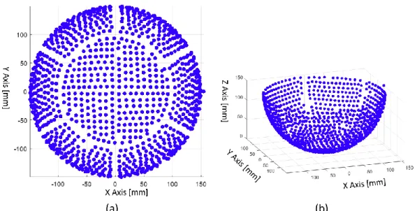
on CT image was utilized to find the fiducial points. ... 24 Fig. 2-6 The pattern of 1024 channels in hemisphere 650 kHz FUS transducer. (a) XY plane

view of the transducer (b) oblique bird eye view of the plotted transducer ... 27 Fig. 2-7 (a) A CAD sketch of transducer, skull assembly, skull frame and top-head reservoir

(b) The sectional view of the skull frame which imbedded 8 fiducial point. (c) The sketch illustrates the relative heights between the geometrical center of fiducial point and the lower face of the skull frame ... 27 Fig. 2-8 Registration of CT image and transducer pattern. (a) Bird eye view of the composite

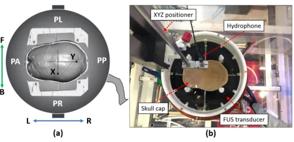
plot of FUS transducer and skull-frame CT image. The fiducial point was painted as red dot (b) A caudal view of the composite plot was illustrated. Note that only half of the transducer channel were plotted ... 30 Fig. 2-9 The coordinate system configuration. (a) The coordinate of hydrophone scanning

domain was marked as front (F), Back (B), left (L) and right (R); The patient perspective direction was plotted as patient anterior (PA), patient posterior (PP), patient right (PR) and patient left (PL); The transducer coordinate was marked using X and Y arrows. (b) The look down view of FUS transducer with skull-frame setup.

(10)

iii

... 30

Fig. 3-1 The simplified model-view-controller (MVC) pattern used in this study. The corel of MVC triangle was maintained to keep the indivisual model independent. The mouse and keyboard listen to the user’s input and interprets this order to the controller. Then the controller manages the predefined work flow and plot the result on the screen to the users. ... 32 Fig. 3-2 Preview of the developed ray tracing software with patient-specific CT and MRI data.

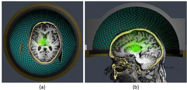
The MR and CT image were registered and the 3D scene could be observed in arbitrary location and angle. ... 32 Fig. 3-3 (a) The 3D illustration of the relative possition between skull structure and wave beam

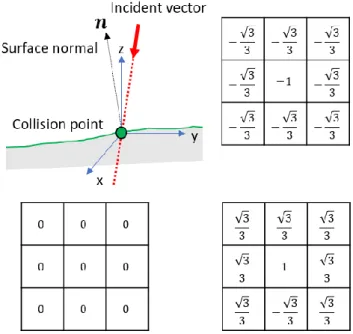
of single transducer channel. (b) The collision detection along ray path. A 0.1mm step size was utilized in collision detection. The brighter pixel represents higher intensity and darker pixel rerpents lower intensity in CT image. ... 36 Fig. 3-4 The surface normal was estimated using 3D Zucker-Hummel edge operator. There

requires three set of basis functions to derive the gradient on XYZ axis. The 3 × 3 × 3 edge basis function, which is gx(x, y, z), for X axis was plotted. ... 36 Fig. 4-1 The penetration of plane wave through water-skull-brain medium. (a) The wave beam

pass through outer and inner layer of the heterogeneous skull bone. (b) The transmission and attenuation loss of plane wave during penetration of skull bone. 41 Fig. 4-2 The attenuation simulation of planar wave in longgitudinal propagation. A

homogeneous medium assumption was defined. A 100 kHz sinusoid signal is utilized and the initial pressrue was 1. The speed of sound was defined as 1540 m/s and α was defined as -200 to visualized a significant decay. ... 44 Fig. 4-3 The sketch of a wave penertrating a boundary between two media. The wave is

(11)

iv

transmitted from a point P through the intersection O and refracted to point Q [63]. The refraction angle is derived with known incident angle and the wave velocity of two materials. ... 45 Fig. 4-4 The three-layer model used in proposed ray method. Two major refractions were

accounted with a homogeneous medium assumption on water-skull-brain model. The closest distacne from target point to the second refracted ray, dx, was treat as the lateral distance from center of the beam. ... 48 Fig. 4-5 The variation of transmission and reflection coefficient while wave propagate from

water to skull was simulated by defining the incident angle as a variable a) The transmission angle based on Snell’s law. b) The variation of transmission coefficient and reflection coefficient. The density and wave speed were defined as 1482 m/s and 1000 kg/m3_{in water, and 3900 m/s and 1900 kg/m}3_{in the skull, respectively. ... 50}

Fig. 4-6 The transmission angle calculated based on Snell’s law while wave propagate from skull to brain with derived transmission and reflection coefficient. a) The transmission angle become saturated while the incident angle is greater than the critical angle b) A uniform amplitude of the coefficient while the incident angle is greater than critical angle was simulated. The density and wave speed were defined as 1482 m/s and 1000 kg/m3_{in water, and 3900 m/s and 1900 kg/m}3_{in the skull, respectively ... 50}

Fig. 4-7 (a) The sketch of scanning plane and selected transducer channel (b) the hydrophone scanned pressure filed and medial filtered pressure field from one of the scaned data. ... 53

Fig. 4-8 The measured pressure decay of single element beam profile. The scaning volume start from focal plane to the closest scannable plane and the total depth of scane was 130 mm. ... 53

(12)

v

Fig. 4-9 The relationship of electrical power and actual acoustic pressure. A saturation of maximum pressure could be observed while the electrical power was greater than 2W. ... 55

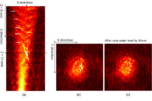
Fig. 4-10 (a) Longitudinal pressure field along beam path of single element, the disturbance pattern captured in hydrophone scaned preesure field were marked as white arrow (b) XY plane pressure field on Z=57 mm depth (c) XY scan after raise water level by 30 mm ... 55 Fig. 4-11 Reconstructed pressure field from hydrophone scanned raw data. The upper row is

longitudinal scan data and lower row is cross-sectional scan data which is the same data as shown in Fig.26. The window size used in four cases were (a) full data (b) 25 sample (c) 20 sample (d) 17 sample. ... 57 Fig. 4-12 The variation of max pixel value based on adopted window size. The shape of beam

is visible start from window size 9 and the water surface reflection is start to appeared when window size larger than 17. ... 57 Fig. 4-13 The sketches of the experiment setup. A single transducer channel was activated to

emit 650 kHz acoustic wave. A robotic arm controlled hydrophone scan was implemented on the focal plane as shown in figure. ... 60 Fig. 4-14 (a) Secure the skull assembly to the top head reservoir which fastened on the top of

the FUS transducer (b) Iteratively move the hydrophone to the corner of the scanning plane to make sure that there is no contact between hydrophone tip and skull bone60 Fig. 4-15 (a) The cross-sectional scan of single element beam without the skull placed between

transducer and hydrophone. The scanning area was 50 mm by 50 mm on XY plane and the scanning depth was 50 mm on Z axis (b) The cross-sectional scan of single element beam with skull placed between transducer and hydrophone. The scanning

(13)

vi

area was 50 mm by 50 mm on XY plane and the scanning depth was 30 mm on Z axis ... 60

Fig. 4-16 (a) Hydrophone measured pressure field on Z=40 mm plane (b) Median filtered pressure field with -6dB contour based on the peak pressure value. ... 63 Fig. 4-17 (a) The beam divergence angle without skull (b) the divergence angle after refracted

by skull bone ... 63 Fig. 4-18 (a) The refraction of beam when targeted at the central location (b) The refraction of

beam when targetting on a frontal target. ... 65 Fig. 4-19 (a) The beam divergence angle without skull attached (b) the divergence angle after

refracted by skull bone ... 65 Fig. 4-20 The simulated focal pattern on 10 different target locations. The color bar was auto-scaled to emphasize the focus. ... 65 Fig. 5-1 The distance from each transducer channel to geometrical center of a hemisphere

transducer. A periodic variation of the distance was visualized. This is an evidence to show the baseline difference of the distance of each transducer from the geometrical center. The geometrical reference was marked using red arrow. ... 69 Fig. 5-2 a) The baseline phase mapping in workstation of InSightec ExAblate neuro system.

The unit of the phase is Radian. b) A customized ‘Z’ letter mapped on transducer pattern in Matlab c) The loaded pattern with the baseline phase in the workstation software. ... 69 Fig. 5-3 The skull bone induced refraction was computed and visualized in developed software

in 3D. The speed of sound in water and skull bone was set as 1482 m/s and 2742 m/s in these two cases. ... 72

(14)

vii

Fig. 5-4The color mapping of computed phase on corresponding channels. The range of the pahse was color mapped in –π to +π. A summation of this pahse map and the baseline phase (see Fig.38-a) caused by manufacturing error was applied before sonication. ... 72

Fig. 5-5 (a)(b) The reconstructed iso-surfaces of two collected skulls. (c) The incident angle θ1 and θ2 in skull 1 setting has smaller value which results better transmission of the propagating wave (d) In contrast, skull 2 has relatively larger incident angle as shown θ3 and θ4. The normal vector of the incident angle was defined as n. ... 74 Fig. 5-6 Pressure field of focal plane measured using a hydrophone. Two different scanning

scales were performed to define a feasible ROI size for a reasonable scanning time with enough coverage of the focal pattern. ... 74 Fig. 5-7 The focal pressure measured on XY and XZ plane with and without skull placed

between transducer and hydrophone. The scanning area is 10 mm by 10mm for all images. a) XY plane without skull b) XY plane with skull c) XZ plane without skull d) XZ plane with skull... 76 Fig. 5-8 A total of 17 sonication with hydrophone scanning were implemented on various

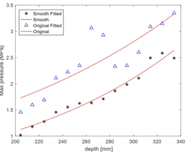
speed of sound in bone for calculating phase delay. ... 76 Fig. 5-9 The improved focal pressure by refraction accounted ray method in skull 1. a) Without

phase correction b) Phase correction without refraction c) Correction with refraction accounted ray tracing d) The comparison of three cases. The pressure of three cases plotted in figure d were represent the pressure lies on the blue line from figure a, b and c. ... 78 Fig. 5-10 The focal improvement using ray tracing based phase compensation on skull 1. A

(15)

viii

Fig. 5-11 The focal improvement using ray tracing based phase compensation on skull 2. A dispersed focal pressure distribution could be visualized in this skull setting. ... 79 Fig. 5-12 The improved focal preassure compared with non-phase corrected case in both skull.

A significant improvement of the focal peak pressure was obtained on skull 2. In contrast, the higher peak pressure was achieved in skull 1 phase compensation. .... 81 Fig. 5-13 The relation between activated channel number and the increased peak pressure. The

decrease of focal pressred is in accord with the decrease of the activate channel in both skull measurement. ... 81 Fig. 8-1 The basic structure of ray tracing platform and the work flow of the developed

software. It is feasible to extend the usage of the software to new designed researches by adding a functional module. ... 91 Fig. 8-2 The captured image from a graphical user interface of the developed ray tracing

software. The activated transducer channel was plotted on the left bottom and the skull density ratio (SDR) was plotted on the right bottom. A varying channel number and SDR could be computed and visualized in real-time frame. ... 91 Fig. 8-3 The mapping of the incident angle corresponding to each transducer. The incident

angles equals or greater than the critical angle were mapped as red disks on the surface of skull where the ray intersects with the outer skull, and the incident angles under critical angle were plotted as green disks. A) The distribution of the incident angles when the sonication target lies on the center of the skull volume. B) The mapping of the incident angles when the sonication target lies on the postal side of the skull ... 94 Fig. 8-4 The transformation of a sphere shape to ellipsoid one. A) The XY plane plot of the

constructed 3D ellipsoidal shape with the original hemisphere B) The XZ plane plot of the constructed ellipsoid with the original hemisphere. ... 97

(16)

ix

Fig. 8-5 The mapping of the incident angle corresponding to each transducer. The incident angles equals or greater than the critical angle were mapped as a red disk on the surface of skull where the ray intersects with the outer skull, and the incident angle ... 97

Fig. 8-6 The activated channel mapping of various ellipsoid shape. The axial ratio from 1 to 0.9 was utilized to design different ellipsoid transducer. ... 98 Fig. 8-7 The contour area ofdifferent contour levels in sagittal plane with the varying ellipsoid

axis ratio. ... 98 Fig. 8-8 The contour area of different contour levels in coronal plane with the varying ellipsoid

axis ratio. ... 100 Fig. 8-9 The contour area of different contour levels in transverse plane with the varying

(17)

1

Chapter 1 INTRODUCTION

Focused ultrasound (FUS) is an attractive technique to noninvasively treat deeply seated brain tissue leaving collateral structure unaltered. Recently, the thermal ablation treatment for essential tremor was approved by Food and Drug Administration (FDA) in the United States and the treatment is commercially available for patients. The main challenge of this technology is the skull bone, which significantly attenuates and scatters the acoustic beam. In addition to experimental approaches, the numerical simulation studies have been highly investigated in the past twenty years, and the technology becomes more matured. Despite its high accuracy of full wave simulation, the long computation time make these techniques not possible to adopt in clinical environment.

The objective of this study is to develop a fast simulation tool based on ray method to compensate skull-induced aberration with a reasonable accuracy. The overarching theme of the studies was improvement in computation time of the phase correction with a more realistic acoustic ray model than the one implemented in clinical system from empirical approach. In this work, emphasis was placed on two factors: the importance of refraction in the phase correction, the impact of wave velocity in the skull bone to the phase correction.

Chapter 2 provides an overview of the focused ultrasound in the brain applications as well as a review of the compensation studies and the treatment protocol used in clinical environment. In Chapter 3 the registration method used in studies is described. In Chapter 4 to 6, the developed ray based software and the experiment evaluation for phase correction was described. The discussion was described in Chapter 7 and the limitations were listed in Chapter 8. Finally, the conclusions were summarized in Chapter 9 and the applicable future studies were listed in Chapter 10.

(18)

2

1.1. Brain tumor

According to the 2014 World Cancer Report, tumors of the nervous system account for less than 2% of all cancers but have a marked impact on cancer morbidity and mortality [1]. Glioblastomas are the most common and most malignant central nervous system neoplasms, for which the three-year survival rate is less than 3% due to their resistance to radiation and chemotherapy [2]. In addition to primary tumors, studies suggest that brain metastases may develop in up to 19% of lung cancer patients [3], 5% of anywhere [3], and 30% of breast cancer patients [4].

Treatment options for brain tumors include surgical removal or destruction of the tumor using heat, radiotherapy, and chemotherapy, or a combination of two or more of the modalities. For surgical treatment, complete or partial resection of the tumor was performed to remove as much as possible. This has all the risk of open surgery, including bleeding, sensory and motor weakness, and neurologic injury. The radiofrequency ablation is the most commonly used nonsurgical treatment for brain tumors. This stereotactic approach typically uses small lesions, which can limit the accuracy of energy delivery and the effectiveness in larger lesions. It also contains all the risks of invasive procedures. As a non-invasive approach the Gamma Knife is very attractive, but the defect is significant [4-6]. Ionizing radiation is problematic, especially in pediatric patients. There is also a delayed response to treatment, risks to long-term cognitive abilities, and oncologic risks. Chemotherapeutic approaches for treatment of brain cancers have the limitation of inability to deliver drug because the blood-brain barrier prevents the drugs from reaching the cancerous cells.

Ultrasound (US) has several advantages, which make it well suited as diagnostic and therapeutic tool in the human tissue. First, it is nonionizing and can be used non-invasively. As a diagnostic modality, ultrasound equipment is less expensive than Computed Tomography (CT) or Magnetic Resonance Imaging (MRI) devices and has the advantage of portability.

(19)

3

These features make it much more accessible, although its usage in the brain is limited because of the skull bone. However, it is possible to circumvent this limit with the help of advanced electrical control and modern computing power. This will be discussed in the following section.

1.2. Skull bone and mathematical models

1.2.1. Wavelength and skull thickness

The use of ultrasound in the brain presents several unique challenges. The skull bone (see Fig. 1-1) is the biggest barrier of ultrasound in the brain. The skull is comprised of an outer layer of dense cortical bone, which encapsulates a porous trabecular bone center. Skull bone is heterogeneous, and has asymmetric geometry.

The longitudinal speed of sound in the skull bone varies with location and frequency, but is on average approximately 2900 m/s [7, 8] twice that of water. Both speed of sound and attenuation increase with increasing density of the trabecular bone [9]. As a result, sound passing through the skull undergoes inhomogeneous phase shifts, resulting in a defocusing of the beam. Refraction effects arising from non-normal incidence of the ultrasound on the skull further distort the beam profile [10].

In addition to dephasing of the beam, the insertion loss of the skull is very high. This is due to a combination of factors. First, the acoustic impedance of bone differs significantly from both water and soft tissue, resulting in high reflective losses at the tissue-bone interface. The reflective losses can vary from approximately 30-80% at normal incidence [7]. At low frequencies (approximately 500 kHz and lower), reflective losses dominate the total loss observed through human skull bone [7]. At higher frequencies scattering and absorption play a greater role, making it very difficult to transmit frequencies greater than 1 MHz through the

(20)

4

skull bone [7]. The absorptive losses raise an additional concern. Because bone absorbs ultrasound energy at a much higher rate than the surrounding tissue, there are the potential hot spots, particularly at the scalp/bone interface where the ultrasound energy is the highest. In therapeutic processes, this means that the temperature at the bone interface could surpass the temperatures achieved at the transducer focus, even when low frequencies are employed [11].

Distortion of the ultrasound beam increases with frequency as the phase shifts become significant relative to the small wavelengths associated with higher frequencies [10]. Multiple reflections can also occur between the transducer and the skull, contributing to phase distortions at the focus [12]. Thus the skull bone presents a major obstacle for therapeutic ultrasound. The following sections will discuss the techniques to compensate the skull-induced aberration.

(21)

5

Fig. 1-1 The wave length vs. the skull bone in CT image. The upper half are micro CT images of fragments of mouse, rat and rabbit skulls showing relative sized and lower half is CT image of human skull bone [10].

(22)

6

1.2.2. Mathematical model

The mathematical models describing the propagation of acoustic waves in biological body can be typically categorized into beam model and full-wave models[13]. The derivation of the equation on each model is outside the scope of this section. Thus, a general overview of these mathematical models will be described.

1.2.2.1. Acoustic beam models

The fundamental concept of acoustic beam models is an approximated mathematical depiction of acoustic wave propagation. It is easier to understand and implement numerically than the full-wave models. The simplicity has resulted in a widespread usage and a large number of proposed extensions and improvements to the original models. The Rayleigh-Sommerfeld (RS) integral and the angular spectrum method (ASM) are the typical methods.

Rayleigh-Sommerfeld model

Two fundamental assumptions were adopted in the RS model: that the vibrating surface of the piezoelectric element, is flat and part of an infinite rigid baffle, and that the generated acoustic waves are propagating within an infinite, homogeneous, linear, and isotropic media [14-16]. Prior to the calculation, the surface of any arbitrarily shaped transducer or array is subdivided into a finite number of point sources. In a similar manner, the area or volume of the medium where the acoustic pressure is required is sampled to a number of observation points. The total acoustic pressure at each point can then be calculated as the algebraic sum of all contributions [16, 17]. Some extensions to improve the shortcoming of original RS model were proposed. The Tupholme-Stepanishen model, more commonly known as the impulse-response model [18, 19] was introduced in order to account for diffraction effects at the edges

(23)

7

of the vibrating piezoelectric element which is not feasible with the original RS model. The layer-based inhomogeneity model complements the original RS model with Snell’s law, thus permitting for reflection and refraction of the acoustic waves to be taken into account [14]. An alternative formulation of the RS model, named the fast nearfield method (FNM), has been proposed to compute the nearfield region in case of simple transducer shapes. This method simplifies the double integral calculation in the RS model to a fast converging single integral, which is then evaluated using Gauss quadrature [20-22].

Angular spectrum method

The ASM model was first introduced in the field of Fourier optics [23]. This model involves the calculation of an acoustic field’s spectral components on an initial plane and propagation of the plane through space by multiplication of each spectral component with an appropriate phase propagation factor [24]. The ASM, usually requires the initial help of the RS model in order to calculate the acoustic wave field from an arbitrary transducer onto a source-plane, and then propagates through its own computation domain. A rapid computation performance could be achieved by permitting of the calculation of the acoustic pressure on an entire plane through a single inverse FFT operation [25]. Various approaches have been proposed to address the majority of limitations restricting the use of the ASM in realistic simulations. The inability to model nonharmonic wavess, e.g., broadband waves or pulses with the ASM could be improved by running separate ASM simulation based on derived frequency components by taking one-dimensional FFT on broadband excitation signals. The summation of each pressure field by an inverse FFT yields the final pressure field [26, 27]. The inability to model wave propagation in heterogeneous media could be overcome by assigning a different speed of sound for each plane where the wave is calculated on [28]. The ASM model does not account for energy loss during its propagation. However, by replacing the real valued wavenumber with a complex number it is possible to account for absorption and attenuation effects [25, 27]. As mentioned

(24)

8

above for RS model, by combining Snell’s law with ASM it is possible to account a refraction effect [27]. The foremost drawback of the ASM method is its inability to model wave propagation in a medium exhibiting 3D spatial inhomogeneities. Recently, a hybrid angular spectrum method (hASM) was introduced to address this limitation [25].

1.2.2.2. Full-wave model

Linear acoustic pressure wave equation

In contrast to an acoustic beam model, a full-wave model provides more accurate and realistic depictions of acoustic wave propagation. The most fundamental full-wave model of acoustic wave propagation is the linear acoustic pressure wave equation (LAPWE) which is derived from three fundamental equations of fluid dynamics. These are Euler’s equation, the continuity equation and the constitutive equation. The Euler’s equation of motion in fluid provides a nonlinear relation between acoustic pressure and particle velocity. The conservation of mass equations, states that the rate of mass flowing into a fixed volume is considered equal to the increase of mass inside the volume. This equation yields a relation between the medium’s equilibrium density and the particle velocity. Being a full-wave model, the LAPWE model can account for all the wave propagation phenomena, which include reflection, refraction, diffraction and scattering. However, there are three major limitations of LAPWE. As this model discards high-order terms, nonlinear propagation phenomena cannot be accounted for. Since this model is derived from fluid dynamics equations, the resulting partial differential equation can only account for longitudinal waves. Another downside to the LAPWE is that it does not account for energy absorption [29-31]. The external force, such as mass injection, body force and turbulence sources could be included in source terms and this method is referred to as a convected LAPWE [24, 32]. The lossy LAPWE model which includes lossy term in the right-hand side of the linear continuity equation is used in the

(25)

9

derivation of LAPWE [29]. The shear wave on skull bone and the nonlinearity near the transducer surface could be accounted by adding an additional elastic Westervelt-Lighthill euation (WLE) model [33].

1.3. Transcranial Focused ultrasound (TcFUS)

1.3.1. Treatable neurological disease using TcFUS

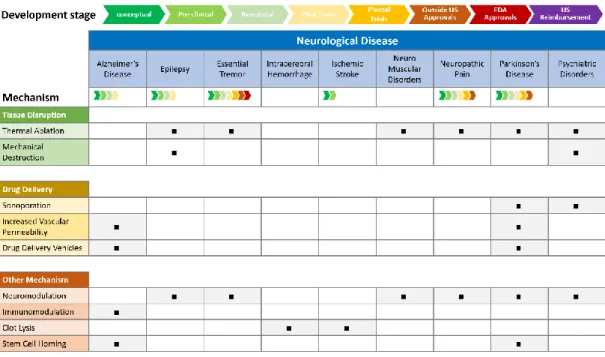
Focused ultrasound is a platform technology that can produce multiple biological effects on pathological brain tissue through either thermal or mechanical means. These effects are dependent on the nature of the tissue (e.g. muscle vs. bone) and the ultrasound parameters (power, duration, and mode-continuous versus pulsed) [34]. The applicable mechanisms using focused ultrasound on neurological disease is illustrated in Fig. 1-2. As Fig. 1-2 shows, thermal ablation and neuromodulation could be utilized as therapeutic means to treat many brain diseases. A large and growing number of clinical applications for focused ultrasound are in various stages of research, development and commercialization [34] and they are summarized in Fig. 1-2. The availability of a variety of biomechanisms creates the possibility of treating a variety of disorders. We do not make any attempt to discuss the detail of each mechanism and its biological effects in this study. An overview of focused ultrasound’s biological effects is introduced in this reference [34].

(26)

10

Fig. 1-2 The development stage of the focused ultrasound on various neurological diseases and corresponding mechanism.

Fig. 1-3 The correction of skull induced phase abberation. The focal spot generated under in phase sonication usualy has a oblique and off-target concentration. A precisely tuned phase delay on each channnel of array transducer could improve the focal spot location.

(27)

11

1.3.2. Focal spot aberration by skull

The foremost barrier when treating the brain with TcFUS is the skull. The complex heterogeneous nature of the skull, which is multi-layered, liquid-filled and porous, causes non-negligible distortion of the focal quality. It is well known that less than 10 percent of the acoustic energy penetrates through the heterogeneous skull structure. Depending on the skull property along the beam path, the wave emitted from each channel in the transducer array experiences a different delay. In this scenario, an in-phase (simultaneous) sonication may cause an unpredictable distortion. As shown in Fig. 1-3, the in-phase sonication through the skull may result in a shifted and distorted focal spot. A nicely tuned phase delay for each channel could shift the focal spot back to targeted location (see Fig.1-3). The technique to refocus the focal spot is called skull compensation or phase correction. Different from other FUS applications in the soft tissue, skull compensation is crucial when treating the diseased target in the brain. In the following section, we will briefly introduce the compensation techniques proposed in the literature.

1.3.3. Skull compensation studies

Focused ultrasound treatment of the brain began in the early 1950s with the precursor works of Professor Fry [35]. Later, FUS treatment with craniotomy was adopted to treat 50 patients affected by Parkinson’s Disease in 1960 [36]. However, easier infection during and after this invasive operation makes it inappropriate for multiple target and repetitive treatment. Another option, using lower sonication frequency and longer wavelength, may minimize the interference of the skull refraction. However, lower frequency also decreases the cavitation threshold, thus leaving a strict requirement for cavitation monitoring and control. Moreover, decreasing the frequency results in enlarged and blurred focal volume, which may decrease

(28)

12

heating precision. As the technology has been developed, the scientists found that a solution to these problems is to use large, multi-element transducer arrays with several hundred to over a thousand elements, where each element is driven with an optimized phase and amplitude. The large transducer surface permits the acoustic energy to be distributed on the skull surface, thus diminishing the local deposition of ultrasound energy on the scalp and bone. The ability to drive the transducer elements individually with appropriately corrected phases and amplitudes allows compensation of focal distortion effects [37].

Previously, the compensation study for skull-induced phase correction ranges from purely analytical or numerical calculations of the required aberration corrections to entirely experimental approaches, with a varying degree of invasiveness, usability, and success. Time reversal techniques, like the implanted hydrophone[38-40] and the ‘acoustic stars’[41], undoubtedly provide the highest refocusing quality. However, this invasive approach could result in undesirable tissue damage and unlikely to be utilized in clinics for multi-targeting treatment. Analytical calculations or simulations to derive phase and amplitude correction are entirely non-invasive and already being employed on modern TcFUS systems. However, despite their speed and ease of use, the purely analytical methods are inherently limited as they do not account for the entire range of wave propagation phenomena[37], unlike full-wave simulation-based techniques. Simulation-based technique [42, 43] can account for most of the physical phenomena, e.g. reflections, refractions and attenuation that occur during wave-propagation, while some models can even account for non-linear wave wave-propagation, cavitation and shear waves. However, the high complexities, heterogeneous anatomical structures and the higher acoustic frequencies may require huge amount of computation resource to allow such simulations to run in viable time frames especially when accounting for non-linearity and shear waves. MR acoustic radiation force imaging (MR-ARFI) [44-46] is entirely non-invasive and has demonstrated the ability to produce high quality focusing. This technique exhibits the unique characteristic of directly monitoring acoustic pressure, and offers the possibility of

(29)

13

closed-loop control of transcranial sonication. Nonetheless, MR-ARFI is still in its initial stage and requires hours of measurement in the presence of the patient and the careful management of the transducer element grouping and activation[37].

The adoption of available technique is highly dependent on the strategy of the manufacturing company and the strategy is highly influenced by the demand from actual users – clinical surgeons. A non-invasive technique with a real-time or quasi-real-time functionality to provide rapid estimation for better treatment planning may increase its adoption rate and be more attractive for clinical usage. From the aforementioned technique, the best scenario is to combine the fast performance of analytical techniques and the accuracy of simulation techniques. However, there is always a trade-off between physical accuracy, simulation time and computational resources. In this study, a ray based phase correction technique was developed to compute pressure to the focal area and its verification was performed using hydrophone measurement.

1.4. The treatment protocol

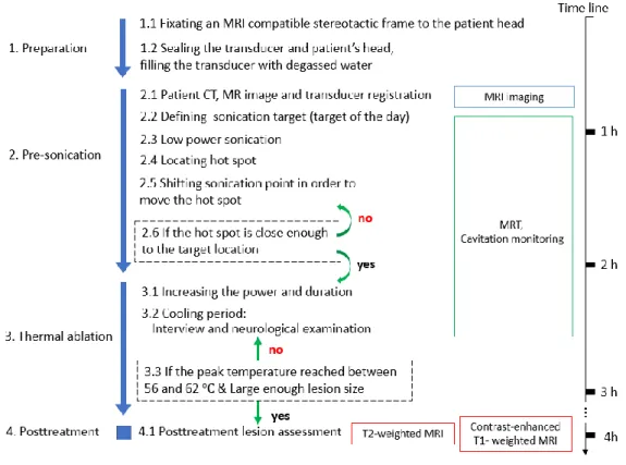
The treatment protocol is well documented in literature [47-49]. The workflow of the treatment protocol is illustrated in Fig.1-4. A treatment flow is summarized with some limitations in this section.

Prior to the treatment day, pre-treatment planning images need to be obtained. These include a CT scan of the entire cranium and an MRI to define the target. These pre-treatment MR images are registered for delineation of the target [48]. On the treatment day, a stereotactic frame is fixed to the patient’s head using local anesthesia. The frame-pins are placed as low as possible over the lateral orbits, just above the eyebrows, and in the occipital bone at or below the level of the external occipital protuberance. A circular elastic membrane with a central

(30)

14

opening is stretched to fit tightly around the head and placed as low as possible on top of the stereotactic frame [48]. This preparation process takes approximately 15 to 30 minutes. After pre-test of the transcranial MR guided focused ultrasound (TcMRgFUS) device using a gel phantom, a patient then is positioned supine, head first on the MR table. The stereotactic frame is locked to the MR table to maintain a constant position between the patient and the transducer [48].

Low power sonication, resulting in sub-therapeutic heating in the 40-45 o_{C range, is}

performed to localize the focal spot using MR thermometry. Phase correction is used to steer the beam within a small range of a few millimeters. For larger changes in focal spot position, the transducer is physically moved, while the patient stays fixed in a frame that is mounted to the MR table and is only in contact with transducer system through the flexible membrane and water [48]. After the focal spot is sufficiently steered to the target, sonication is performed with sufficient power to achieve a planned target temperature such as 55-60 o_{C. During the}

cooling periods of several minutes between each sonication treatment, magnetic resonance images may be acquired. Moreover, since the patients are fully awake during the entire intervention procedure, the cooling period are used for interviews and neurological examinations [47]. Both optimal coverage of the target and clinical feedback from patients play a role in determining treatment. Total treatment time spent on the MR table, including positioning, imaging, planning, sonication and post MR imaging is typically four hours. This could be fallen to as low as 2 hours of table time in some experienced centers, not including frame placement and post-operation imaging.

(31)

15

(32)

16

The abovementioned treatment time is typically for an ideal case. The treatment time can easily be extended for various reasons. An unintentional movement of the patient during sonication could rewind the treatment to the initial registration stage which could easily take an additional hour to shift the focal spot of the target. Due to individual differences, the thickness and acoustical properties of the skull are significantly different between patients. The phase correction is estimated from the path of each ray crossing the skull from the transducer elements to the focus [48]. However, difficulty elevating peak temperature on thick skull cases has been reported and the skull density ratio showed a positive relation to the peak achievable temperature [50]. A planning tool, with fast computation of phase correction and is based on a more realistic acoustic model could circumvent the limits. The treatment could be accelerated and the untreatable target could be ablated using optimization of transducer-patient placement with a fast simulation tool.

(33)

17

Chapter 2 MATERIALS AND EXPERIMENT SETUP

In this chapter, the hardware setup of the experiment will be presented and the software-hardware registration process described in detail. The experiment was implemented at the Focused Ultrasound Center at the University of Virginia.

2.1. Experiment preparation-hardware setup and system wiring

The degassed water (the remaining oxygen level less than 1.1%) was prepared using collected tap water before wiring the hardware system. The treatment bed (Fig.2-1.3) was undocked from the MRI system and moved toward the door of MR room with the power cable connected to the transducer amplifier (Fig.2-1.4). The FUS transducer (Fig.2-1.2) was carefully detached from the treatment bed and placed in the AIMS III scanning tank (AST3-L, ONDA, CA, US). The transducer was mounted on a purpose built frame which was fixed inside of the scanning tank in order to keep the transducer face up and rigidly fixed. The scanning tank was kept waterless during whole experiment and the transducer was filled with degassed water. The portable degassing suitcase (Fig.2-1.7) was utilized as a pump to feed the degassed water into the transducer. During the experiment, the FUS work station (Fig.2-1.8) was utilized to setup the inputs of each sonication.

(34)

18

Fig. 2-1 Hardware system setup and wiring. ①3T GE MRI imaging system ② InSightec, ExAblate 650 kHz focused ultrasound transducer ③ Focused ultrasound patient treatment bed ④ Amplifier of transducer ⑤ XYZ positioner ⑥ Positioner guide system ⑦ Portable degassing suitcase ⑧ Work station of FUS system ⑨ Control PC of MRI imaging system ⑩ Machine room

Fig. 2-2 The skull frame to mount the skull into the FUS transducer. (a) Superior and (b) left view of skull-frame (marked as ①) mount (c) Superior and (d) left view after connect skull-frame to assembly base (marked as ②), four 40mm long connecting rod was utilized to connect the skull-frame to assembly base

(35)

19

2.2. Skull-frame setup on the FUS transducer

The cadaver skull was mounted on a polycarbonate frame using four polyvinyltoluene (PVT) screws from four directions (Fig.2-2.a) and then put into a degassing cylinder. One-hour skull degassing was performed before attaching the skull-frame to the assembly base. Four 40 mm connecting rods were utilized to secure the skull-frame on the assembly base and then the whole assembly was kept in the degassed water. A silicone grease was smeared on the groove of transducer edge and the top-hat reservoir (in Fig.2-2.2, white container) was attached on the transducer.

2.3. Supporting pad removal on the CT image

A skull-frame image volume was acquired using the CT scan feature in a Gamma system (Leksell Gamma Knife Icon, Elekta Inc, CA, US) with the CBCT setting as shown in Table 1. A supporting pad was placed under the skull-frame during CT imaging in order to level the frame to the X-axis of the CT image. Undesired voxels were also captured in this CT image because of this supporting pad. The skull frame CT image will be utilized in ray tracing simulation and the voxels formed by the supporting pad may provide incorrect refraction of the ray tracing. These voxels are required to be removed and a filtered version of the CT image was created. A semi-automatic image processing algorithm was developed using an active mask to remove undesired voxel in CT images. The boundary of the active mask was interactively calculated based on manually defined seed points on each image frame. First, one central seed point needs to be defined which requires approximate placement on the center of the skull cap in CT image. Then, two seed points which were placed few pixels below the bottom face of the frame need to be defined and this will give an angle limitation for the edge

(36)

20

searching process (Fig.2-3.a). A searching ray may emit from the defined central seed point and across the skull cap until reaching a defined length. The number of rays was arbitrarily defined as 9 and it can be changed depending on the requirement. The intensity along each ray was collected. A simple peak finding process provides the inner and outer layer location of the skull from the intensity data. The outer layer is used as a minimum guide to the active tracing edges.

Since the skull cap has a non-linear shape and radius is changing along the horizontal axis in sagittal plane (Fig.2-3.b), the tracking edge could be defined by adding an amount of pixel value to the detected inner edge on Sagittal plane. In order to derive the tracking edge from detected inner skull layer an ellipsoidal fitting was applied to get a smooth cap shape. In addition, the ellipsoid cap was shifted by few pixels to make a guideline for the tracing edge computation in the coronal plane (Fig.2-3.c). A guide line was used as the radius of the tracing edges and the final mask was formed based on the tracing edges, manually defined seed points and the bottom boundaries of the image below two seed points. The processed image was saved as a new series of DICOM images and the 3D surface was reconstructed per the following section.

Table. 1 The cone beam computed tomography (CBCT) setting for skull-frame CT imaging in Leksell Gamma Knife Icon system

CTDI [mGy] Voltage [kV] Current [mA] Pulse Length [ms] Number of projections 6.3 90 25 40 332

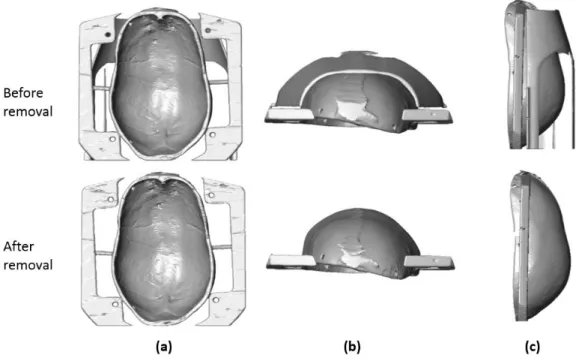
The 3D structure of the skull with a frame was reconstructed using the isosurface function in the medical image processing software Amira 5.2 (FEI Visualization Sciences Group, Bordeaux, France) and the reconstructed surfaces before and after removal were illustrated in Fig.2-4.

(37)

21

Fig. 2-3 The work flow of support pad removal from the CT image (a) Three seed points were manually defined (two white star point and one yellow star point). The red star points denote the actively tracked edge points which will utilized as boundary of the removal mask (b) The detected inner layer of skull cap was marked using red dots (c) A ellipsoidal shape fitting was applied on the detected skull layer and shifted a certain distance to create a guide line to the active tracker on Coronal plane

Fig. 2-4 The reconstructed skull-frame volume from CT image before and after remove the supporting pad (a) cranial view (b) frontal view (c) lateral view

(38)

22

2.4. Fiducial point coordinate in CT image

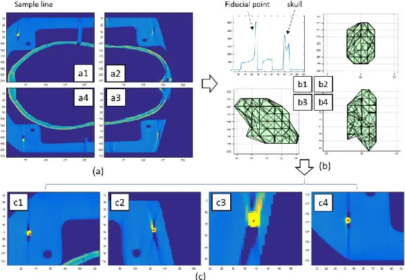
The fiducial points in CT images have distinct and relatively large voxel intensity and a known image volume. These features can be utilized while computing the central position of fiducial points in the image coordinates. An image processing technique (Fig.2-5) was developed for finding and localizing the centroid of the fiducial points imbedded in the skull mounting frame from a computed tomography (CT) image volume.

The default DICOM series data were stored as consecutive images on coronal plane as shown in Fig. 2-5.a. Since the fiducial points within the skull mounting frame were placed at a parallel plane to the transverse plane of skull, it is more convenient to process the image on the transverse plane. The DICOM images were imported in computer memory using Matlab and the transverse plane images were separated to four parts to ensure that each of them contains one fiducial point (Fig. 2-5.a). The fiducial point with highest pixel value (brightest) was visible on the corner of the skull mounting frame (Fig. 2-5.a1~a4). A threshold based edge searching algorithm was implemented on four separated image volumes and a sample line (vertical dashed line in Fig. 2-5.a1) to show the intensity difference between different materials was plotted in Fig. 2-5.b1. The threshold was defined as 5850 based on the pre-investigation on three cutting planes (on Sagittal, Coronal and Transverse plane) which all intersect the fiducial point. The intensity of the fiducial points in this version of CT image has a saturated maximum value of 6000 and this limits the precision of central location detection based on pure image intensity. A candidate 3D volume for a fiducial point could be reconstructed based on the detected threshold-based edges as shown in Fig. 2-5.b2~b4. It assumes that the geometrical center of this 3D edge volume represents the fiducial point. The derived fiducial points (red dot) with the closest CT image plane were shown in Fig. 2-5.c. The CT image derived fiducial points are listed in Table 2. However, these coordinates need to be transformed to a measurement based coordinate system and this will be discussed in a following section.

(39)

23

Then a registration between the skull-frame structure and FUS transducer could be achieved by using a derived transformation matrix.

Table. 2 CT image derived fiducial point coordinate in CT image domain. The voxel size is 0.5ⅹ0.5ⅹ0.5 mm3_. This coordinate serves as ananchor to allow the registration between different systems.

Point # X axis Y axis Z axis

P1 31.0831 73.2729 298.9306

P2 349.9560 59.1668 306.3435

P3 363.7277 378.8297 304.7568

(40)

24

Fig. 2-5 The image process to localize the fiducial points in CT image. A threshold of 5843.3 on CT image was utilized to find the fiducial points.

(41)

25

2.5. Fiducial point coordinate in transducer system

An INI configuration file is placed in the ‘ExportData’ folder on InSightec workstation. This configuration file contains information about the 3D location and surface area of each transducer channel. S portion of the geometry data is shown in Table 3.

Table. 3 Portion of 650 kHz FUS transducer geometry file. Total of 1024 channel coordinates and surface areas were stored in an INI configuration file in the workstation folder ‘\EportData\XX-XX-XX_ANx\WSFiles\Site\SiteInifiles\XdIni’

The numerical simulation estimates the focal quality of the FUS sonication and requires a detailed geometry of each element in the transducer. The data stored in the configuration file provides such information, and it can be used in the reconstruction process to define transducer geometry which can be subsequently utilized as a boundary condition of numerical simulations. The pattern of transducer elements on two different views was plotted in Fig.2-6.

Based on the CAD sketch (Fig.2-7.a) of the transducer, the skull mounting frame and the top-hat reservoir, it is possible to derive the central coordinate of fiducial points. Eight fiducial points were imbedded in the skull-mounting frame. However, only four fiducial points were visible in the skull-frame CT image. This is an artifact of a small scan volume of the Leksell Gamma Knife CT scanner. A CT scanner with larger scan volume is desirable to provide a full capture of the skull-frame structure. This would also increase the accuracy of registration with the help of eight, rather than four, registered fiducial points from CT.

Channel # 3D Coordinate [mm] Surface Area X Y Z Square [mm^2]

XCH0 82.5241 7.8761 24.8625 124

XCH1 72.302 7.8012 18.6807 124

XCH2 61.1608 7.9406 13.1391 124

(42)

26

The coordinates of a fiducial point on X and Y axes (horizontal plane) could be easily derived from a measured schematic of the FUS transducer setup, but the relative heights between fiducial centroid and the transducer are not described in the sketch. Since we know that the radius of the fiducial points is 1mm, the length from fiducial centroid to lower plane (Fig.2-7.b) of the skull-mounting frame could be geometrically derived as shown in Fig.2-7-c. Note that, the detailed geometry of actual FUS transducer was not permitted to be distributed and is not included in this paper because it is considered to be protected corporate intellectual property. Fig. 2-7.a is a simplified sketch and it does not represent the actual scale of FUS transducer. Finally, the fiducial point coordinates in the FUS transducer domain were derived and listed in Table. 4.

Table. 4 Fiducial point coordinate derived from transducer CAD and measurement.

Point # X coordinate Y coordinate Z coordinate

P1 -80 80 137.3

P2 80 80 137.3

P3 80 -80 137.3

(43)

27

Fig. 2-6 The pattern of 1024 channels in hemisphere 650 kHz FUS transducer. (a) XY plane view of the transducer (b) oblique bird eye view of the plotted transducer

Fig. 2-7 (a) A CAD sketch of transducer, skull assembly, skull frame and top-head reservoir (b) The sectional view of the skull frame which imbedded 8 fiducial point. (c) The sketch illustrates the relative heights between the geometrical center of fiducial point and the lower face of the skull frame

(44)

28

2.6. Skull-frame CT and FUS transducer registration

Since the voxel size (0.5ⅹ0.5ⅹ0.5 mm3_{) of CT was precisely defined and the unit of}

transducer coordinate is in millimeter, the transformation between CT and transducer data is much simpler and only the rotation matrix may be involved.

In linear algebra case, the singular value decomposition (SVD) is a factorization of a real or complex matrix. Formally, the singular value decomposition of an m by n real or complex matrix M is a factorization of the form UΣV*_{, where U is an m by m real or complex unitary} matrix, Σ is a rectangular diagonal matrix with non-negative real numbers on the diagonal, and V is an n by n real or complex unitary matrix [51, 52].

𝑀 = 𝑈Σ𝑉∗ _(2.1)

In the special, when M is an m by m real square matrix with positive determinant, U, V*

and Σ are real m by m matrices as well, Σ can be regarded as a scaling matrix, and U, V*_can be viewed as rotation matrices. Thus, the expression 𝑈Σ𝑉∗_{can be intuitively interpreted as a} composition of three geometrical transformation; a rotation or reflection, a scaling, and another rotation or reflection.

Since, the data size of transducer is much smaller than the CT image it is more efficient to define transducer coordinate as A matrix. The SVD was computed in Matlab software using a SVD function as bellow,

[𝑈, 𝛴, 𝑉] = SVD(𝐹𝑃_𝐶𝑇, 𝐹𝑃_{𝑇𝑟𝑎𝑛𝑠𝑑𝑢𝑐𝑒𝑟}) (2.2) where FP indicates the fiducial point coordinate.

(45)

29

𝑅 = 𝑈𝑉∗ (2.3)

and translation matrix

𝑇 = −𝑅 ∙ (𝐴𝑐𝑒𝑛𝑡𝑟𝑜𝑖𝑑)′+ (𝐵𝑐𝑒𝑛𝑡𝑟𝑜𝑖𝑑)′ (2.4) were computed and the final transformation was implemented based on following formula

𝐵 = 𝑅 ∙ 𝐴′_{+ 𝑇} _(2.5)

Finally, a composite figure of CT skull-frame image and transducer element was plotted in Fig.2-8. In order to give a better see-through view, only half of the transducer was plotted intentionally. This result may contribute a better localization and understand of in-vitro skull experiement and also provide a geometrical configuration of experiment setup for numerical simulation.

2.7. Further coordinate configuration

The coordinate configuration between software-hardware systems was investigated to provide a clear lookup data. As shown in Fig.2-9.a, this configuration combined a coordinates system of the transducer in workstation, patient perspective direction, and hydrophone scanning domain in AIMS system. This configuaration provides key imformation to the hardware-software registration in the follwing study .

(46)

30

Fig. 2-8 Registration of CT image and transducer pattern. (a) Bird eye view of the composite plot of FUS transducer and skull-frame CT image. The fiducial point was painted as red dot (b) A caudal view of the composite plot was illustrated. Note that only half of the transducer channel were plotted

Fig. 2-9 The coordinate system configuration. (a) The coordinate of hydrophone scanning domain was marked as front (F), Back (B), left (L) and right (R); The patient perspective direction was plotted as patient anterior (PA), patient posterior (PP), patient right (PR) and patient left (PL); The transducer coordinate was marked using X and Y arrows. (b) The look down view of FUS transducer with skull-frame setup.

(47)

31

Chapter 3 RAY TRACING SOFTWARE

3.1. The infrastructure of the software

A user-friendly software was developed to visualize the rays on the focal target from transducer elements and to compute the pressure near the focal area. In this chapter, the basic concept of the developed software is presented. The infrastructure of this software was developed by Dr. Snell and Mr. Quigg in Focused Ultrasound Foundation (Focused Ultrasound Foundation, Charlottesville, Virginia, US) at its early stage [53]. This dissertation is an extension of the software to include pressure computation and experimental verification of this software.

In computer graphics, ray tracing is a technique for generating an image by tracing the path of light emitted from a source through each pixel in an image plane and simulating the effects of its encounters with virtual objects [54, 55]. The technique is capable of producing a high degree of visual realism may be used in an analogous way to simulate a wide variety of acoustical effects, such as reflection and refraction, scattering, and dispersion phenomena [56].

The software platform to perform the ray tracing was developed using Java language in NetBeans IDE (Oracle Corporation, Redwood City, CA, US). The main and heavy computation was solved in the graphics processing unit (GPU) using an open graphics library (OpenGL, Silicon Graphics, CA, US). OpenGL is a cross-language, cross-platform application programming interface (API) for rendering 2D and 3D vector graphics. The API is typically used to interact with a GPU to achieve hardware-accelerated rendering and computation.

(48)

32

Fig. 3-1 The simplified model-view-controller (MVC) pattern used in this study. The corel of MVC triangle was maintained to keep the indivisual model independent. The mouse and keyboard listen to the user’s input and interprets this order to the controller. Then the controller manages the predefined work flow and plot the result on the screen to the users.

Fig. 3-2 Preview of the developed ray tracing software with patient-specific CT and MRI data. The MR and CT image were registered and the 3D scene could be observed in arbitrary location and angle.

(49)

33

The software was designed to strictly obey the objective oriented programming (OOP) protocol, which provides a highly flexible and extendable feature. A clear model-view-controller (MVC) pattern (see Fig.3-1) was implemented to separate the coherent connection between each functional module. As shown in Fig.3-1, the triangle connection of MVC pattern provides a flexible foundation to appended modules.

An action listener was designed to pass corresponding attribute to the MVC domain by interpreting the user’s input through mouse and keyboard. The instant parameter and the data generated in the MVC pattern was processed by central processing unit (CPU) and this process occupies the memory in the random-access memory (RAM). On the contrary, the CT and MRI data was loaded directly into the memory in the GPU to reduce the computation load from CPU. The vertex shader and fragment shader was coded in OpenGL shading language in order to project the 3D data to 2D screen. A compute shader was utilized to contain the main computation work as well as the ray tracing algorithm. Furthermore, the manual registration on CT and MRI data could be achieved in developed software. Thanks to the flexibility of the software, it is possible to append more functional modules. Such as the manual registration module for MRI and CT image and treatment data replay module. The source code of this software, expect for the proprietary module of the manufacturer, will be available as an open source project. Thus, the details about the code are not included in this dissertation. A preview of the developed domain is illustrated in Fig.3-2.

In the following section, the basic of computer vision techniques to implemented ray tracing are introduced. The intersection point detection between wave beam and skull surface, and the skull surface normal vector estimation are described.

(50)

34

Since the emitted plane wave is propagated along a beam in the medium, the path of the wave can be illustrated as a line as shown in Fig.3-3.a. After a period of time, the wave may arrive at the skull surface and define a collision point on the skull. However, in reality a large contact area between wave front and skull surface is involved. In this study, we only consider the collision point (marked as green point in Fig.3-3.a) lying on the central axis of the beam, and the skull as well as the subcutaneous tissue were neglected during collision detection.

The source location (beam star point) 𝑝𝑖(𝑥, 𝑦, 𝑧) could be extracted from the transducer parameter INI file created by the system manufacturer. A geometric center oriented vector 𝑣⃑(𝑖, 𝑗, 𝑘) was utilized to represent the wave beam and illutrsated using red dot line in Fig. 3-3.b. The small integer or span of gradient was defined as 0.1 mm. The coordinate of the vector end point 𝑝_𝑖,𝑛 could be defined as follow

𝑝_𝑖,𝑛= 𝑝_𝑖+ 0.1 × 𝑛 × 𝑣⃑ (3.2.1) The corresponding CT value 𝑓_(𝑝

𝑖,𝑛) on the point 𝑝𝑖,𝑛 was collected and compared to the

predefined threshold 𝜏_{𝑠𝑘𝑢𝑙𝑙} which binarizes the CT data to skull and non-skull volume. An iterative increase of 𝑛 was utilized to search the collision point that satisfies 𝑓_(𝑝

𝑖,𝑛)≥ 𝜏𝑠𝑘𝑢𝑙𝑙.

The detected collision represents the intersection between wave beam and skull outer layer. The similar concept was utilized to detect the second collision that represents the intersection point between inner layer and refracted wave beam. Care should be taken while defining the skull threshold because the proposed collision detection method is highly sensitive to this value.

3.3. Surface normal estimation

The surface normal based on pre-detected collision point is crucially required to compute incident angle that will serve in refraction angle computation (Fig.3-4). One might expect that