Spacecraft Precision Attitude Determination using UVF Measurements

(1)

1. INTRODUCTION

system using on-board estimation algorithm. Thus the user can simply use the estimated attitude information as the measurement for the real-time or the ground attitude determination algorithms. On the other hand, UVF output provides the unit vectors of the identified stars and thus the user may select stars used for the attitude determination algorithm. The main advantage of using UVF measurements over QUEST measurements is that the attitude determination performance can be more easily expectable due to the only identified stars are used for the estimation and, in result, the performance improvement can be achieved more systematically.

Spacecraft Precision Attitude Determination using UVF Measurements

Hungu Lee

*

, Jae-Cheol Yoon

**

, and Dongseok Shin

*

*_{Satrec Initiative Co. Ltd., 461-26 Jeonmin-dong, Yuseong-gu, Daejeon 305-811, Korea} (Tel : +82-42-365-7524; E-mail: [email protected])

**_{Korea Aerospace Research Institute, 45 Eoeun-dong, Yuseong-gu, Daejeon 305-333, Korea}

Abstract: This paper proposes a novel approach of a precision attitude determination algorithm using UVF (Unit Vector Filter)

measurements. The proposed method is superior to the conventional QUEST measurements based approaches because the estimation performance can be greatly enhanced by selecting brighter stars having better noise characteristics. The performance comparison with QUEST measurements is made to verify the usefulness of the proposed algorithm.

Keywords: Precision Attitude Determination, UVF (Unit Vector Filter) Measurement, QUEST Measurement

Recent development in remote sensing technology has brought out the need of much more accurate attitude information during the imaging period for the provision of value-added image products. In general, the real-time on-board estimation of a spacecraft attitude does not satisfy the accuracy requirement because a linearized attitude dynamics must be adopted due to the limited computational capability of the on-board processor and the lack of ancillary information. The restitution of accurate attitude information is, therefore, generally carried out at ground stations and it is called the precise attitude determination (PAD) algorithm.

This paper proposes a novel approach of implementing of UVF measurements to attitude estimation algorithms. A PAD algorithm with the UVF measurement is developed for general sensor mounting configuration. The estimation performance is evaluated by using simulated sensor outputs [1] for an imaging situation of an LEO (low Earth orbit) imaging satellite and compared with the results of using QUEST measurement. The results show that the PAD performance using UVF measurements is superior to the QUEST measurements because the performance can be improved by selecting brighter stars having better noise characteristics.

The precise attitude determination with the accuracy of tens of arc-seconds (resulting in several tens of meters geo-location accuracy) is still challenging due to several factors; e.g. the high-frequency variation and perturbation of the attitude dynamics as well as the noise and stability characteristics of attitude sensors currently available. Therefore, the improvement of attitude determination accuracy is essential in order to achieve a comparable amount of ultimate geo-location uncertainty to the orbit determination.

The development of a PAD algorithm and software includes many technological aspects such as the precise modeling of attitude dynamics and sensor characteristics, the implementation of an attitude estimator such as a batch least square estimator, an extended Kalman filter or an unscented Kalman filter, and the analytic and/or experimental determination of noise parameters. Among them, the sensor output characteristics have direct impact on the estimation performance regardless of the estimation method or the dynamic model of the spacecraft.

2. DEFINITION OF COORDINATES

The definitions of coordinate systems are identical with [1]. The satellite is assumed to have a main imaging payload of a push-broom type. The optical bench frame (OBF) of the satellite is thought to be the mechanical body frame. The satellite’s attitude information is, therefore, defined as the OBF attitude with respect to an inertial celestial reference frame (CRF) such as J2000 coordinate. Let’s denote the roll, pitch and yaw rotational angles as φ, θ, and ψ, respectively. Then the 3-2-1 Euler rotational matrix from CRF to OBF is expressed as:

Two types of sensor data are generally used for the attitude estimation: gyro output providing the inertial rate information of the spacecraft and the star sensor output providing the accurate attitude of the spacecraft with respect to an inertial coordinate system. Gyro output characteristic mainly has effect on the stability performance, which is related with the image quality. On the other hand, the star sensor outputs are mainly concerned with the geo-location accuracy number, which is generally treated as a performance index of a PAD algorithm.           + − + + + − − = = θ ψ φ θ ψ φ ψ φ θ ψ φ ψ θ ψ φ θ ψ φ ψ φ θ ψ φ ψ θ φ θ φ θ ψ θ φ ψ θ φ c c s s c c s c s c s s c s s s s c c c s s s c s s c c c C C OBF CRF OBF CRF ) , , ( , x ) , , ( xOBF CRF G G (1)

Another expression of the rotational matrix of (1) using the attitude quaternion is expressed as [2].

Most of the conventional star sensors provide two types of measurement information: QUEST and UVF. QUEST output is the estimated quaternion attitude information of the

spacecraft with respect to the on-board star catalog coordinate 

        + + − − − + + + − + − − − + + − − = 2 4 2 3 2 2 2 1 4 1 3 2 4 2 3 1 4 1 3 2 2 4 2 3 2 2 2 1 4 3 2 1 4 2 3 1 4 3 2 1 2 4 2 3 2 2 2 1 ) ( 2 ) ( 2 ) ( 2 ) ( 2 ) ( 2 ) ( 2 ) q ( q q q q q q q q q q q q q q q q q q q q q q q q q q q q q q q q q q q q COBF CRF (2)

(2)

Two star trackers are mounted on the satellite with different bore-sight directions to compensate the poor angular accuracy around the bore-sight axes. The two star tracker coordinates are denoted as SCF1 and SCF2, respectively, and the rotational matrix from OBF (as the body frame) to SCF1 and SCF2 are specified as:

          − − − − − = 64278761 . 0 41721771 . 0 64245893 . 0 0 83867057 . 0 54463904 . 0 76604444 . 0 35008722 . 0 53908705 . 0 1 SCF OBF C           − − = 64278761 . 0 41721771 . 0 64245893 . 0 0 83867057 . 0 54463904 . 0 76604444 . 0 35008722 . 0 53908705 . 0 2 SCF OBF C (3)

The rotation between OBF and SCF can also be expressed as quaternion as: [ ] [ ] [ [ ]T OBF SCF T SCF OBF T OBF SCF T SCF OBF q q q q 86898579 . 0 25740532 . 0 40521473 . 0 12003007 . 0 86898579 . 0 25740532 . 0 40521473 . 0 12003007 . 0 25740532 . 0 86898579 . 0 12003007 . 0 40521473 . 0 25740532 . 0 86898579 . 0 12003007 . 0 40521473 . 0 2 2 1 1 − − = − = − − = − = ] (4)

The satellite has an inertial reference unit (IRU) measuring the satellite’s body rate. The IRU has four sets of gyros, providing a full 3-axis inertial rate measurement with a redundancy. The relation between the IRU assembly coordinate system, or GCF (gyro coordinate system), and the four gyro measurement directions is specified as:

                        − − − − − = =             = GCF z GCF y GCF x GCF ABCD GCF D C B A ABCD _C ω ω ω ω ω ω ω ω ω 1 0 0 0 3 1 6 1 2 1 3 1 6 1 2 1 3 1 3 2 G G ₍₅₎

The mounting direction of the IRU with respect to OBF is specified as:           − − = = 1 0 0 0 1 0 0 0 1 OBF GCF GCF OBF C C (6) 3. EQUATIONS OF MOTION

The linearized 6-state equation of motion for attitude determination is expressed as [3]             +            − × =       r a v v I I q I q dt d η η δ δ ω δ δ G G 0 0 b 0 0 ] ˆ [ b 2 1 2 1 (7) where

[

ω

ˆ

×

]

is the matrix expressing the vector cross

product and defined as:

          − − − ≡ × 0 ˆ ˆ ˆ 0 ˆ ˆ ˆ 0 ] ˆ [ x y x z y z ω ω ω ω ω ω ω (8)

qv is the vector part of the quaternion error

and q * ˆq q q≡ ⊗

δ

*_{is the conjugate quaternion of q having the following}

characteristics T q q q q_⊗ *₌ *_⊗ ₌[0,0,0,1] ₍₉₎

The conjugate quaternion expresses the inverse rotation of the original quaternion. _rare the rate white noise and rate random walk noise, respectively. They are mutually independent white Gaussian random processes having the following statistical characteristics:

aη η , 3 2 3 2 _, _{ _} } { I E I EηaηaT =σa_rate ηrηrT =σr_rate G G G G ₍₁₀₎

The gyro bias error vector is defined as:

g

g bˆ

b

b≡ −

δ (11)

qˆ

is the estimated quaternion and

ω

ˆ

is the body rate vector having the following relation with the drift bias vector

g gm

bˆ

ˆ

≡

ω

+

ω

(12)

where

ω

_gmis the body rate vector measured by IRU.

The 6-state equation of motion shall now be extended to include absolute GCF misalignment and scale factor error [4] by the following assumptions:

1. The GCF misalignment vector is defined as the difference between ground measured mounting direction, ,and the actual in-orbit mounting direction, , as 0 0 GCF OBF C GCF OBF C 0 ] [ ) ( 3 1 0 0 0 0 ≡ = − × − GCF GCF OBF GCF OBF GCF GCF C C I C

δ

(13)

2. The four gyros mounted in IRU have only diagonal scale factor errors and the scale factor error matrix is thus defined as the following diagonal matrix:

            ≡ Λ D C B A λ λ λ λ 0 0 0 0 0 0 0 0 0 0 0 0 (14)

3. The IRU contains rate integration gyros and thus the gyro output is the accumulated rate information. Then the gyro output vector is expressed as

ABCD r ABCD g dt d ABCD a ABCD g OBF GCF OBF GCF ABCD GCF ABCD gm v v C I C I = − − × − Λ + = angle angle b b ]) [ ( ) ( 0 0 0 δ θ θ (15)

where and are angle white noise and angle

random walk noise, respectively and their standard deviations are ABCD a v a ABCD r v

σ

and

σ

_r.

The extended equation of motion shall be derived from the body rate expression. Thus the angle output equation of (15)

(3)

where shall be approximated as the following rate output equation by

applying the finite difference method:

              =              − × − × − Ω =             =             ∆ ∆ = ∆ 4 3 4 2 1 2 1 2 1 2 1 0 0 0 0 0 ) ( 0 0 0 0 0 0 0 0 0 0 0 0 ] [ ] ˆ [ ) ( , b I I I C t G C C C t F q x OBF ABCD ABCD gm OBF ABCD GCF gm OBF GCF OBF ABCD OBF GCF r a ABCD GCF ABCD g v ω ω η η η η η λ δ δ δ λ G G G G G ABCD r ABCD g dtd ABCD a ABCD g OBF GCF OBF GCF ABCD GCF ABCD gm I C I C η η ω δ ω G G = − − × − Λ + = b b ]) [ ( ) ( 0 0 0 (16)

The new noise characteristics are related with the angle output noise characteristics as:

4 4 2 2 4 4 2 2 2 } { 2 } { × × ∆ = ∆ = I t E I t E r T ABCD r ABCD r a T ABCD a ABCD a σ η η σ η η G G G G (17) G GCF

η

and ηG are white Gaussian noise processes having _λ

their covariance matrices as 2 ₄, respectively.

3

2 _I _, _I

GCF σλ

σ

Now by assuming that the misalignment and scale factor error values are very small, (16) is expressed as

4. STAR SENSOR MEASUREMENT MODELS

ABCD gm OBF ABCD GCF gm GCF OBF GCF ABCD a ABCD g ABCD gm OBF ABCD ABCD a ABCD g ABCD gm GCF ABCD GCF OBF GCF ABCD a ABCD g ABCD gm GCF ABCD GCF OBF GCF OBF C C C I C I C I C I C ω ω δ η ω η ω δ η ω δ ω Λ − × + + + ≈ + + Λ − × + ≈ + + Λ + × − = − − 0 0 0 0 0 0 0 0 0 0 ] [ ) ( ) )( ( ]) [ ( ) ( ) ( ]) [ ( 1 1 b b b

The star sensor misalignments do not affect satellite’s attitude and are only related with measurements. Thus there is no dynamic coupling between star tracker misalignments with (22) when they are augmented into the equation of motion.

where, . The last two terms of the above

equation is expressed as ABCD gm GCF ABCD GCF gm C

ω

≡ 0 GCF GCF gm OBF GCF GCF gm GCF OBF GCF C C [

δ

]

ω

0[

ω

]

δ

0 0 0 × =− × ABCD D gm C gm B gm A gm ABCD gm ABCD ABCD gm OBF ABCD ABCD gm OBF ABCD diag C C λ ω ω ω ω λ ω ≡ ≡ Ω Ω = Λ G G ), , , , ( , 0 0

[

]

T D C B A λ λ λ λ

The star sensor misalignment vector is calculated from the error quaternion between ground measured nominal mounting direction and the in-orbit mounting direction as:

      ≅ 1 2 1 0 SCF SCF SCF q δ (23)

and thus the following relation is obtained. _{Two star sensors are assumed to be mounted on the spacecraft} and thus two misalignment vectors are assumed to have the following statistical characteristics:

ABCD a OBF ABCD ABCD ABCD gm OBF ABCD GCF GCF gm OBF GCF ABCD g OBF ABCD ABCD gm OBF ABCD OBF C C C C C η λ δ ω ω ω G G 0 0 0 0 0 0 _b _[ _] + Ω − × − + ≈ (18) 2 2 1 1 SCF ,dtd SCF SCF SCF dtdδ η δ η G G ₌ = (24)

The estimated body rate is obtained from (18) as _{Now by defining the following error vectors}

2 2 2 1 1 1 SCF ˆSCF , SCF SCF ˆSCF SCF δ δ δ δ δ δ ≡ − ∆ ≡ − ∆ (25) ABCD ABCD gm OBF ABCD GCF GCF gm OBF GCF ABCD g OBF ABCD ABCD gm OBF ABCD OBF C C C C λ δ ω ω ω ˆ ˆ ] [ bˆ ˆ 0 0 0 0 0 G Ω − × − + ≡ (19)

the augmented equation of motion is now expressed as η′ ′ + ′ ∆ ′ = ′ ∆x F(t) x G(t) dt d ₍₂₆₎

From the small angle rotation assumption, the quaternion error vector is related with the Euler angle error as

where ) ˆ ( , ₂1 2 1δθ δ ω ω δqv= dtd qv= − (20)       = ′       = ′           = ′           ∆ ∆ ∆ = ′ ∆ × × 6 6 6 6 2 1 2 1 ) ( ) ( 0 ) ( ) ( , I t G t G t F t F x x SCF SCF SCF SCF η η η η δ δ G G and from the following definitions

ABCD ABCD ABCD GCF GCF GCF ABCD g ABCD g ABCD g λ λ λ δ δ δ ˆ ˆ bˆ b b G G G − = ∆ − ≡ ∆ − ≡ ∆ (21)

The star sensor measurement equation is defined as the attitude of CCD array of the star sensor with respect to the inertial coordinate system(CRF) as:

the extended equation of motion is obtained as η ) ( ) (t x Gt F x dt d_∆ ₌ _∆ ₊ ₍₂₂₎

(4)

        ∆ − × ∆ − ∆ + = − − − − − − − − − 1 | 1 | 1 | 2 1 1 | 1 | 1 | 2 1 1 | 2 1 1 | 1 | ˆ ˆ ˆ 1 ˆ ˆ ] ˆ [ ˆ ˆ ˆ 0 0 0 k k v k k SCF OBF T k k SCF k k v k k SCF OBF k k SCF k k SCF k k v k k SCF OBF q C q C q C δ δ δ δ δ δ 0 0 0 0 OBF CRF SCF OBF SCF SCF SCF CRF q q q q = ⊗ ⊗ (27)

Now we derive the measurement equation expression for the

UVF measurement and QUEST measurement. _{Now by ignoring the second order terms with respect to the}

state variables, the vector term of the QUEST measurement residual is obtained as:

4 .1 QUEST Measurement

The QUEST measurement is the quaternion determined by the on-board algorithm of the star sensor. The measurement residual is defined as QUEST k SCF v SCF OBF k k SCF SCF QUEST k C C q n z = 0 _|₋₁ 00

δ

+21∆

δ

+ ˆ G ₍₃₁₎

The measurement sensitivity matrix is then expressed as:

* 1 | 1 | ˆ ) ˆ ( 0 0 0 − ⊗ ⊗ − ⊗ ≡ kk SCF OBF k k SCF SCF QUEST k QUEST k q q q q z (28)         = − − 3 2 1 1 | 2 2 3 2 1 1 | 1 1 0 0 0 0 ˆ 0 0 0 0 ˆ 0 0 0 0 0 0 I C C I C C H _SCF OBF k k SCF SCF SCF OBF k k SCF SCF QUEST k (32)

where is the QUEST output of the star sensor and is the a priori quaternion estimate obtained by integrating quaternion kinematics with the initial condition of

. Also q is the estimate of and is

expressed as QUEST k q 1 | ˆkk− q | 1 ˆ_k_{− k}₋ q 1 ˆ 0k_|k−₁ SCF SCF SCF SCF q 0

The above expression is identical with the result of [4].

4 .2 UVF Measurement

The UVF measurement utilizes the identified star information. The advantage of the UVF measurement is that the noise characteristics of all three axes of the unit vectors toward the identified stars are uniform regardless of the apparent angle between the star sensor’s boresight direction. Thus the UVF measurement residual is defined as

1 | 1 | 2 1 1 | 0 0 0 0

ˆ

1 ˆ

− − −

⊗

≡













≈

k k SCF SCF SCF SCF SCF SCF k k SCF k k SCF SCF

q

δ

(29) UVF k k k k UVF k w w n zG ≡ ˆ − ˆ _|₋₁+ (33) Now (28) can be expressed as

where, is the true unit vector is SCF and is related with the corresponding star unit vector in CRF, , as

k wˆ k vˆ

(

) (

)

| 1 * 1 | 1 | 1 | * 1 | * 1 | * 1 | * * 1 | * 1 | 1 | ˆ ˆ ˆ ˆ ˆ ˆ ˆ ˆ ) ˆ ˆ ( 0 0 0 0 0 0 0 0 0 0 0 0 0 0 0 0 0 0 0 0 0 0 0 0 0 − − − − − − − − − − ⊕ ⊗ ⊗ ⊗ ⊗ = ⊗ ⊗ ⊗ ⊗ = ⊗ ⊗ ⊗ ⊗ ⊗ = ⊗ ⊗ ⊗ ⊗ ⊗ = k k SCF OBF k k SCF SCF SCF OBF k k SCF SCF k k SCF SCF k k SCF SCF SCF OBF k k SCF OBF SCF SCF k k SCF SCF SCF OBF k k true SCF OBF SCF SCF k k SCF OBF k k SCF SCF true SCF OBF SCF SCF QUEST k q q q q q q q q q q q q q q q q q q q q q q q z δ δ δ wˆk =CCRFSCFvˆk (34)

and

n

UVF_k is the measurement noise.

Now, by expressing the rotational matrix as the exponential matrix, (34) becomes where

(

)

(

)

k OBF CRF SCF OBF SCF k OBF CRF v SCF OBF k OBF CRF SCF OBF k OBF CRF v SCF OBF SCF k OBF CRF SCF OBF SCF SCF k v C C v C q C v C C v C q I C I v C C C w ˆ ˆ ] [ ˆ ˆ ] 2 [ ˆ ˆ ˆ ˆ ] 2 [ ] [ ˆ ˆ 0 0 0 0 0 0 0 0 0 0 0 0 0 0 0 0 × − × − ≈ × − × − ≈ = δ δ δ δ * 1 | 1 | 0 0 0 ˆ ˆ ₋ = ⊗ SCF_k_k₋ SCF SCF SCF k k SCF SCF q q q

δ

and the operator is defined as the inverse operator of the quaternion multiplication as [4]

⊕

where is the spacecraft’s attitude matrix using the estimated attitude quaternion( ) and the second order terms with respect to the state variables are ignored similarly with the case of the QUEST measurement. Also,

0

ˆ

OBF CRF

C

qˆ

      = ⊕ ⊗ ⊕ = ⊗ 1 0 0 ] ][ [ 1 2 2 1 q C q q q q q q (30) k OBF RF C SCF OBF SCF k OBF RF C SCF OBF SCF SCF k SCF CRF k k

v

C

I

v

C

v

C

w

ˆ

])

ˆ

[

(

ˆ

0 0 0 0 0 0 0 0 1 |

×

−

≈

=

≡

−

δ

Then the QUEST measurement residual is expressed as

              ∆ − ∆ × ∆ − =                     − × − =       × = − − − − − − − − − − − − − 1 ˆ ˆ 1 ˆ ˆ ] ˆ [ 1 ˆ 1 0 0 ˆ 1 ˆ ˆ ] ˆ [ ˆ 1 0 0 ˆ ] ˆ [ 1 | 1 | 1 | 2 1 1 | 2 1 1 | 2 1 1 | 1 | 1 | 1 | 1 | 1 | 1 | 1 | 0 0 0 0 0 0 0 k k v k k SCF OBF T k k SCF k k SCF k k SCF k k v k k SCF OBF T k k v SCF SCF k k v SCF SCF k k v SCF SCF k k k k SCF OBF k k SCF SCF QUEST k q C I q C q q q I q C q z δ δ δ δ δ δ δ δ δ δ _{Thus (33) is expressed as}

(

)

UVF k SCF k OBF CRF SCF OBF v k OBF CRF SCF OBF UVF k k OBF CRF SCF OBF SCF k OBF CRF v SCF OBF UVF k n v C C q v C C n v C C v C q C z + ∆ × + × = + × ∆ − × − ≈ δ δ δ δ ] ˆ ˆ [ ] ˆ ˆ [ 2 ˆ ˆ ] [ ˆ ˆ ] 2 [ 0 0 0 0 0 0 0 0 0 0 0 0 G (35)

(5)

(

)

(

)

      × × × × = ] ˆ ˆ [ 0 0 0 0 ] ˆ ˆ [ 2 0 ] ˆ ˆ [ 0 0 0 ] ˆ ˆ [ 2 0 0 0 0 0 0 0 0 0 0 0 0 2 2 1 1 k OBF CRF SCF OBF k OBF CRF SCF OBF k OBF CRF SCF OBF k OBF CRF SCF OBF UVF k v C C v C C v C C v C C H (36)

5. A SIMULATION RESULT

The performance when using the UVF measurement for the precision attitude determination is compared with the case of using the QUEST measurement. Sensor output and dynamics simulation are based on the implementation method expressed in [1]. The applied estimation method is the extended Kalman filter (EKF).

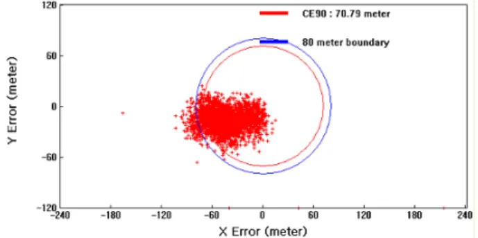
Figure 2 6-State Geo-location Error (EKF+UVF)

5 .1 6-State Estimation using EKF _{As expected, the localization error using the UVF}

measurements is superior to the case of using the QUEST measurements. The mean star magnitude of the UVF measurements is about 2.5 which gives smaller NEA (noise equivalent angle) than the QEUST measurements.

The 6-state estimation performance using EKF based on the dynamic model of (7) is shown in Table 1, Table 2, Figure 1 and Figure 2. Three UVF vectors are used for the estimation using the UVF measurements. The stars are ordered by its magnitude and only the three brightest stars are used.

5 .2 Full State Estimation using EKF

The estimation performance using EKF based on the full state dynamics of (26) is shown in Figure 3, Table 3 and Table 4.

Geo-location Error (CE90 = 226.13 m)

RMSE (m) STD (m) Min (m) Max (m)

X 198.46 20.53 -273.87 -127.11

Y 25.24 23.01 -94.05 40.70

Pointing Accuracy (arcsec)

RMSE STD Min Max Yaw 9.63 3.46 -3.22 19.69 Pitch 14.97 13.50 13.17 25.89

Roll 57.17 6.13 39.28 80.04

X 47.50 20.10 -165.69 14.58

Y 20.68 12.00 -63.22 23.82

RMSE STD Min Max Yaw 11.66 4.29 -27.07 2.93 Pitch 3.88 3.60 -13.59 11.66

Roll 14.86 5.60 -1.75 48.90 Table 1 6-State Estimation Performance (EKF+QUEST)

Table 3 Full State Estimation Performance (EKF+QUEST)

Figure 1 6-State Geo-location Error (EKF+QUEST)

Figure 3 Full State Geo-location Error (EKF+QUEST)

X 99.08 42.36 -151.14 15.93

Y 29.95 16.70 -69.09 15.77

RMSE STD Min Max Yaw 18.84 10.74 -30.21 10.98 Pitch 5.21 5.21 -13.22 11.17

Roll 30.23 10.37 6.08 44.27

X 43.79 9.93 -129.46 -14.47

Y 27.82 11.49 -12.60 54.78

RMSE STD Min Max

Yaw 6.97 2.16 -12.78 12.89

Pitch 11.52 2.46 3.31 18.55 Roll 10.13 2.34 2.88 36.49 Table 2 6-State Estimation Performance (EKF+UVF)

Table 4 Full State Estimation Performance (EKF+UVF) When the number of stars used for the UVF measurements are

(6)

increased from three to four, the localization error is greatly enhanced to 35.30 m as shown in Table 5.

X 18.44 13.95 -129.02 25.39

Y 13.80 9.51 -37.40 31.08

RMSE STD Min Max Yaw 2.84 2.78 -6.57 11.94 Pitch 3.47 2.99 -12.23 15.64 Roll 5.87 3.55 -4.57 36.11

Table 5 Performance Enhancement using Four Stars (EKF+UVF)

5. CONCLUSIONS

A novel derivation of using the UVF measurement which can be applied to the ground processed precision attitude determination algorithms is proposed. The usefulness of using the UVF measurements over the QUEST measurements is demonstrated in a simulation result. The estimation performance when using the UVF measurements can be enhanced by increasing the number of the stars used for the estimation. However, the performance enhancement is expected to be saturated as the number of stars increase. Also it is expected that even the performance may be degraded because less brighter stars having worse noise characteristics are used for the estimation. Thus it is necessary to analyze the estimation performance with increasing number of stars used for the estimation together with the computational load, which is remained as a future research topic.

ACKNOWLEDGMENTS

The works in this paper was supported by KOMPSAT system integration department of KARI (Korea Aerospace Research Institute), Daejeon, Korea.

REFERENCES

[1] H. Lee, J.-C. Yoon, Y.-J. Cheon, D. Shin, H. Lee, Y.-R. Lee, H.-C. Bang, and S.-R. Lee, “Simulation of Spacecraft Attitude Measurement Data by Modeling Physical Characteristics of Dynamics and Sensors,”

ICCAS 2004, The Shangri-La Hotel, Bangkok, Thailand, August 25-27, 2004.

[2] J. R. Wertz, Spacecraft Attitude Determination and

Control, Kluwer Academic Publishers Group, Dordrecht, Holland, 1978.

[3] E. J. Letterts, F. L. Markley and M. D. Shuster, “Kalman Filtering for Spacecraft Attitude Estimation,” Journal of

Guidance, Control, and Dynamics, Vol. 5, No. 5, pp. 417-429, 1982.

[4] M. E. Pittelkau, “Kalman Filtering for Spacecraft System Alignment Calibration,” Journal of Guidance, Control,