Appl. Sci. 2020, 10, 8727; doi:10.3390/app10238727 www.mdpi.com/journal/applsci Article
An Integrated Approach to Real-Time Acoustic
Emission Damage Source Localization in Piled Raft
Foundations
Yong-Min Kim 1, Gyeol Han 1, Hyunwoo Kim 2, Tae-Min Oh 3, Jin-Seop Kim 4 and Tae-Hyuk Kwon 1,*
1 Department of Civil and Environmental Engineering, Korea Advanced Institute of Science and Technology
(KAIST), Daejeon 34141, Korea; [email protected] (Y.-M.K.); [email protected] (G.H.)
2 Deep Subsurface Research Center, Korea Institute of Geoscience and Mineral Resources (KIGAM),
Daejeon 34132, Korea; [email protected]
3 Department of Civil and Environmental Engineering, Pusan National University (PNU),
Busan 46241, Korea; [email protected]
4 Radioactive Waste Disposal Research Division, Korea Atomic Energy Research Institute (KAERI),
Daejeon 34057, Korea; [email protected]
* Correspondence: [email protected]
Received: 21 October 2020; Accepted: 2 December 2020; Published: 5 December 2020
Abstract: Acoustic emission (AE) has garnered significant interest as a promising way to detect the
early-stage development of internal cracks and damage in underground and geotechnical structures, associated with natural disasters. Meanwhile, AE source localization techniques that can identify the damage location in a piled-raft foundation (PRF) are premature because of its complex geometry, although the PRF is a widely used deep foundation type for high-rise buildings. In this study, we propose an integrated approach to localize AE sources in the PRF by using the modified Akaike information criterion (AIC) method and examine its accuracy to mark with pile zones. We performed a series of experiments on a scaled PRF model at a ratio of 1:50, composed of one raft and 25 piles. The results demonstrate that the combined approach with the modified AIC method and the Simplex method can localize the AE source zones with good accuracy, greater than 95% on average. The suggested two-stage AIC picker shows accurate onset time determination, and hence, it significantly improves the accuracy, particularly effective for the signals with low signal-to-noise ratios. The approach exploiting the two-stage AIC picker can be readily used for automated real-time AE monitoring to detect crack generation and its location in buried foundations that cannot be inspected visually.
Keywords: source localization; acoustic emission; damage; non-destructive test; piled-raft
foundation; real-time monitoring; onset time
1. Introduction
The initiation and growth of cracks within a material release energy through the re-distribution of stress [1–3]. This energy is rapidly emitted in a form of transient elastic waves propagating spherically from a localized source. The elastic wave in a particular frequency range from 1 kHz to 1 MHz is referred to as the acoustic emission (AE). Accordingly, AE waves emitted during crack initiation and growth can be captured with acoustic sensors attached on the material surface [4,5]. The deployment of an array of multiple sensors enables to locate AE sources based on the arrival time differences of AE signals at different sensor locations. This allows real-time AE monitoring of target structures while capturing a time-dependent damage process [6–8].
Meanwhile, real-time and non-destructive structural health monitoring (SHM), which continuously monitors in-service structures and localizes the weakened area in structures, has garnered significant interest in association with frequent occurrences of natural disasters and geohazards [2,9,10]. In particular, it is difficult to characterize the damage or defects in underground structures, such as building foundations buried in the subsurface, which are not able to be inspected visually. While it is important to detect the early-stage development of internal cracks, the AE method has been proven as an effective and promising tool for real-time SHM of underground and geotechnical structures. Extensive efforts have been made to apply the AE techniques at a field scale for underground and geotechnical structures, including mines, tunnels, geothermal engineering, and radioactive waste repositories [2,7,10–13].
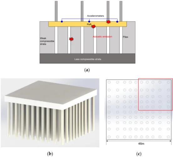
A piled-raft foundation (PRF) is most widely used for high-rise buildings. However, there have been limited attempts on the AE source localization in the PRF. It is a challenging task because the PRF has a complex geometry composed of a mat (or raft) and a group of piles, as depicted in Figure 1. On the other hand, the precise determination of the onset time of the AE signal has the most pronounced contribution to the accuracy of AE source localization [14–16]. A group of cracks is simultaneously developed, and thus multiple AE signals are released within a short time frame. Manual determination of the onset time of each signal is time-consuming and less feasible. Additionally, its accuracy can be subjected to the performer’s experience. Therefore, automation of onset time determination is one of the critical components in developing real-time AE monitoring while not compromising the accuracy of source localization. Previously, various methods for automatic AE onset time determination have been proposed, which include the fixed amplitude threshold method, short-term average/long-term average (STA/LTA) method, Hinkley criteria, Akaike information criterion (AIC) picker method [17–20]. However, these automated methods have hardly been implemented nor used for a PRF structure with complex geometry.
(a)
(b) (c)
Figure 1. (a) Monitoring of structural damage at a piled-raft foundation (PRF), and (b, c) schematic
In this study, we propose an integrated approach combining the modified Akaike information criterion (AIC) method and the Simplex method to localize AE sources in the PRF. We performed a series of experiments on a scaled PRF model at a ratio of 1:50, which was composed of one raft and 25 piles, and explored the feasibility of using a fully automated three-dimensional source localization method on the PRF model. The AE signals were artificially generated by using Hsu–Nielsen source at three different locations—raft top surface, raft bottom surface, and middle of a pile. We compared the accuracy of the source localization between the conventional AIC method and the modified two-stage AIC method. The conventional single-two-stage AIC method requires the setting of a time window to capture the onset time, but it is difficult to use a pre-determined window size when the signal-to-noise ratio is low and the rising of the wave is not clear [21]. To overcome this limitation, the two-stage AIC method was applied at the predetermined time window based on the result of the single-stage AIC method. The location of AE sources was computed based on the onset time with the Simplex method. The discussion on the effect of signal quality and field implementation follows.
2. Model and Test Setup
2.1. Scaled Model for Piled-Raft Foundation (PRF)
A square-patterned PRF with a side length of 46 m was modeled and scaled at a ratio of 1:50, as shown in Figure 1b,c. The scaled PRF model was manufactured with high-density polyethylene (HDPE). The HDPE has a density of 930–970 kg/m3, tensile strength of ~14 MPa, Young’s modulus of
~290 MPa [22–24]. We measured the P-wave velocity VP of the HDPE material as 2450 m/s and the
rod wave velocity VRod as 1600 m/s. Accordingly, the other elastic wave velocities can be also
calculated; the shear wave velocity VS = 950 m/s, the Rayleigh surface wave velocity VRayleigh = 780 m/s, and the dynamic Poisson’s ratio νdynamic = 0.42. Owing to the symmetric characteristic of the modeled
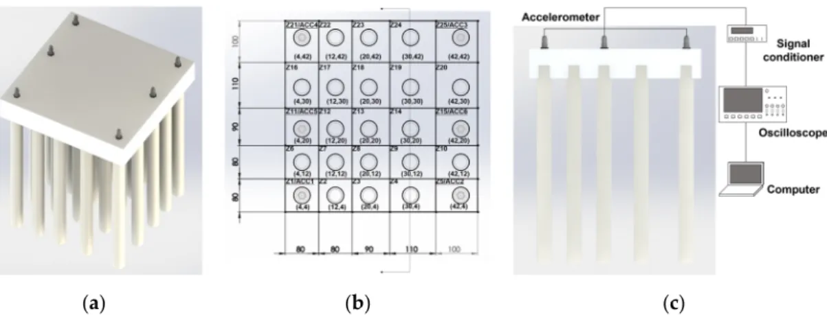
PRF, one-quarter plane of the PRF was fabricated, as shown in Figure 2a. Thereby, the model PRF included 25 piles on which caps were threaded and connected to a raft on them. The spatial arrangement of the pile was asymmetrically patterned in the quarter plane, as it accounts for structural load distribution from the super-structure. The overall dimension of the model PRF was 460 mm × 460 mm × 80 mm in length, width, and height. The piles had a cylindrical shape with a diameter of 40 mm and a height of 500 mm. Figure 2b details the locations of the piles and accelerometers in the model PRF. In addition, the raft was divided into 25 tessellated zones by using the Voronoi diagram, which allocates the zones to the closest pile.
(a) (b) (c)
Figure 2. A schematic diagram of (a) a scaled PRF model, (b) the location of pile foundation and
2.2. Setup for Signal Generation and Acquisition
Artificial AE signals were generated by using the Hsu-Nielsen (H-N) pencil-lead break method, in which the pencil lead is pressed against the surface until the lead breaks [25]. For the consistent AE signal generation, the pencil lead with 3 mm length and 0.5 mm diameter was firmly pressed against a surface at 30° degree to the surface until the lead broke. The H-N pencil lead break generated an intense acoustic signal, which had similar characteristics with the actual AE signal in concrete, and this is considered as a point AE source [26,27]. The H-N pencil lead break method is widely used in AE experiments to verify coupling between AE sensors and a specimen surface, AE attenuation, and source localization capabilities, due to its good reproducibility [27–29].
The generated artificial AE signals were captured at six accelerometers (353B18, PCB piezotronics) which had a sensitivity of 10 mV/g and the operating and resonant frequencies of 0.0035–30 kHz and > 70 kHz. In fields, it is difficult to install a sensor array on the buried foundation in the subsurface. Therefore, we attached the accelerometers on the upper surface of the raft by using vacuum grease to provide acoustic coupling and mechanical fixtures. The array of accelerometers was spatially arranged to cover the whole area of the raft foundation, as shown in Figure 2b.
The AE signal captured by each accelerometer was simultaneously conditioned and amplified with the gain level of 40 dB through a signal conditioner (482C series, PCB piezotronics). The conditioned AE signal was recorded at a sampling interval Δt of 60 ns, and a total of 31,250 data points per signal was acquired by the 8-bit A/D converter (or digital oscilloscope, DSO-X 3024A, Agilent technologies). We used two oscilloscopes and two signal conditioners to cover six accelerometers at the same time. Thereby, the signals simultaneously captured at the six accelerometers were synchronized to share the same time stamp for source localization. Our testing condition in the laboratory had low levels of mechanical and electronic background noises. Therefore, we directly used the acquired raw signals for AE source localization without any signal filtering and preprocessing.
2.3. Experimental Program
A series of experiments with H–N pencil lead breaks were conducted to examine AE source localization in the 3D model PRF. We applied the H-N pencil lead breaks at three different locations— raft top surface (or RT), raft bottom surface (or RB), and pile middle at a distance of 10 cm from the raft bottom (or PM). Additionally, a total of 15 piles installed on the half surface of the raft was tested, exploiting the symmetry—Zones #1 to #5, #7 to #10, #13 to #15, #19, #20, and #25 (Figure 2c). A total of 45 cases (15 piles at each location) were examined. Moreover, we repeated the test 20 times per case to produce sufficient data and assess accuracy.
Figure 3 shows the representative AE wave signatures and their frequency spectra, where the artificial AE sources were generated from the three locations in Zone 14, and the AE signals were captured by ACC1. The majority of the AE energy was placed from 5 kHz to 20 kHz, whereas a clear decrease in the amplitudes was confirmed with an increase in the travel distance.
Figure 3. Acoustic emission (AE) signals acquired at three different locations: (a) time-domain signals
and (b) frequency responses. Note that RT, RB, and PM indicate that a source was generated at the raft top, raft bottom, and pile middle. The AE sources were produced at Zone 14.
2.4. Single-Stage and Two-Stage AIC Method for Onset Time Determination
The Akaike information criterion (AIC) was implemented for automatic onset time determination. The AIC function based on the autoregression (AR) model divides a signal into two vectors at the time k, and compares the signal variance of prediction errors before and after the time
k in a predetermined time window [15,19,30]. The proper time window size is required for precise
onset time determination [21]. The equation of AIC function is expressed as follows:
AIC( )
k
=
k
log(var( [1, ])) (
x k
+ − − ⋅
S k
1) log(var( [
x k
+
1, ]))
S
, (1) where S is the last sample of the time series, k increases from 1 to S through all samples of x, var denotes the variance function, and var(x[1,k]) indicates that the variance of x from the first x1 to k-th xk. The k value with the minimum AIC value is determined as the onset time of the AE signal tmin[15,31].
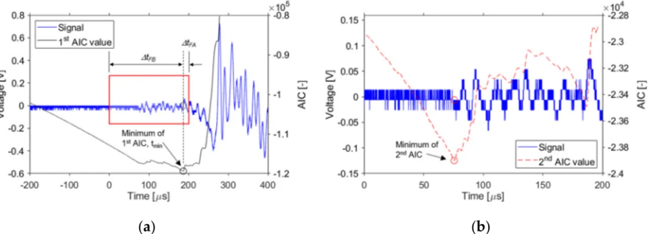
In this study, the single-stage AIC method adopted the time window that started from the beginning of the original signal and ended at the maximum amplitude of the signal. In addition, the two-stage AIC method was applied to improve the accuracy of AE source localization. The two-stage AIC method consisted of two rounds of the AIC picking [32,33]. The single-stage AIC method was carried out as the first round of AIC picker, as shown in Figure 4a. Thereafter, the second round of AIC picker was applied with a narrower time window with a constant size (Figure 4a). The arrival time difference was less than ~200 μs at the farthest accelerometer from the source in this particular case with the used material and the PRF geometry. Accordingly, the window size was fixed to be 200 μs (Figure 4a). The onset time picked in the first round of AIC (tmin)was used as the reference point at each signal. For a fixed window size, the time interval from the beginning of the window to tmin is
ΔtFB, and the rest of the window is ΔtFA, such that the total window size is ΔtFA+ΔtFB. The window
lengths before and after the onset time picked in the first round of AIC tmin, ΔtFB, and ΔtFA were determined as 8 μs and 192 μs, respectively, in all the cases. ΔtFA was assigned to be 8 μs to increase the effectiveness of the second-round AIC picker. The rest of the window was determined to be ΔtFB.
(a) (b)
Figure 4. The two-stage Akaike information criterion (AIC) method for estimation of an onset time of
an acoustic emission signal: (a) the first-round estimation, (b) the second-round estimation. The vertical (voltage) resolution and the horizontal (time) interval in the 8-bit A/D converter were approximately 19.5 mV and 60 ns for this acquired signal.
The k value with the minimum AIC value in the second round defines the onset time of an AE event, as shown in Figure 4b. This two-stage AIC method was applied for the cases with inaccurate AE source localization with the single-stage AIC method.
2.5. Localization Algorithm of AE Events: Simplex Method
The time difference in the determined onset times at two different accelerometers can be computed and the set of these time differences enables the estimation of AE source location with a given wave velocity of the medium. For AE source localization, we used the Simplex method, which is a kind of time-of-arrival localization method. This method is widely used due to its robust convergence characteristic. The Simplex method searches the minimum value of the mathematical functions by comparing the function value at each vertex in the space, taking advantage of specific iterative rules [11,12,34,35].
The error E can be calculated for an arbitrary point within the medium by comparing the computed onset time differences with the AIC-based onset time differences. Accordingly, the error value E is computed at every point in space, which is called error space. Herein, we determined the mean square error (or L2 norm error) as the error value E. Finally, the point with the minimal error is localized as the source location of the AE event [35]. The L2 norm error was calculated every 1 mm interval in the x-y plane, as follows:
2 − − − = −
i i i i t tt t tt n n E m q , (2)where E is the L2 norm error, ti and tti are the onset time determined by AIC picker and the calculated
arrival time at ith accelerometer, respectively, n is the number of accelerometers, m is the number of equations, and q is the degree of freedom. Meanwhile, the z-coordination for the AE source, or the depth z, was fixed according to the artificial AE signal location. This simplified the source localization as the 2-D problem. In this study, we used the constant, pre-determined depth value: z = 4 cm, which is the middle depth of the raft thickness for all the cases.
The source localization requires the medium wave velocity V as an input. Therefore, the representative wave velocity values for the RT, RB, and PM cases were found by using the Hsu-Nielsen (H-N) pencil-lead break and the accelerometers in the scaled PRF model. With four accelerometers attached to the top surface of the PRF, the artificial AE sources were generated on the raft top, the raft bottom, and the pile middle. For the RT and RB cases, the first arrival captured in the accelerometers corresponded to P-wave. Therefore, the RT and RB cases used the P-wave velocity VP
of 2450 m/s. Herein, the P-wave velocity VP was determined with the time-difference-of-arrival
(TDOA) method. For the PM case, the wave propagates through a pile with no confinement, which corresponds to the rod wave propagation. Therefore, the rod wave velocity VRod of a cylindrical HDPE rod was determined using the free-free resonant column (FFRC) method, and this VRod value of 1600 m/s was used for the PM case.
We evaluated the accuracy of source localization by two approaches: Euclidean distance error and zonation based on the Voronoi diagram. First, the Euclidean distance error (EDE) was determined by calculating a distance from the estimated source location to the exact source location. Second, tessellated zones were produced by the Voronoi diagram to assign one pile to each zone. The accuracy was determined by comparing the estimated zone and the actual pile zone. Herein, the accuracy was expressed as a percentage point, based on 20 trials.
3. Results and Analyses
3.1. Localization of AE Event Sources: Single-Stage AIC Result
Figure 5a presents a typical set of the acquired AE signals, in which the onset times estimated by the single-stage AIC method are superimposed. Due to the high signal-to-noise ratio (SNR), the single-stage AIC picker estimated the onset time with a good level of accuracy. Figure 5b shows the estimated source location and the error contour plot estimated by the Simplex method. Our source localization result shows that the estimated source location was (29.3 cm, 18.8 cm) for the actual
source location of (30 cm, 20 cm). Out of twenty trials, the average Euclidean distance error was 1.73 cm, and the zonation was correctly predicted for Zone 14 with Pile #14.
(a) (b)
Figure 5. (a) The onset times determined through the single-stage AIC method, and (b) the spatial
distribution of variances computed by using the Simplex method. Note that the AE source was generated at Zone 14 (30,20) on the raft top (RT) of the model PRF. The amplitude of each signal was normalized with its peak amplitude for comparison.
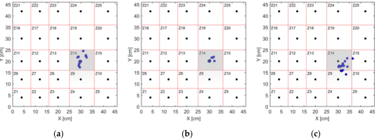
Accordingly, the estimated source localization can be plotted for each AE event. Figure 6 shows the spatial distributions of the estimated source locations using the single-stage AIC picker and the Simplex method when the source was located in one of the central zones (Zone 14). The suggested algorithm resolved most of the trials for RT and RB cases in the central zones. The average accuracy for the RT and RB was recorded to be 93.3% and 100%, with the average Euclidean distance error (EDE) of 1.92 and 0.77 cm, respectively (Table 1). By contrast, the PM case showed poor accuracy of 66.67% with the EDE of 4.68 cm, mainly attributable to the reduced SNR because of the longer travel distance from the source to the accelerometers. This needs further refinement in the onset time determination.
(a) (b) (c)
Figure 6. Localized sources estimated using the single-stage AIC method when the hit sources were
far within the sensor network (or central region): when a hit was applied (a) on the raft top, (b) under the raft bottom, and (c) at the middle of Pile #14. In (c), the middle of the pile at a distance 10 cm down from the top of the raft was struck.
Table 1. The results of source localization estimated by single-stage and two-stage AIC.
Location Zone#
Single-Stage AIC Two-Stage AIC
EDE (cm) Zonation Accuracy (%) EDE (cm) Zonation Accuracy (%) Raft top Corner 2 8.24 25% (5/20) 0.87 100% (20/20) 3 1.95 100% (20/20) 0.48 100% (20/20) 4 2.06 100% (20/20) 1.24 100% (20/20) 10 2.29 100% (20/20) 1.03 100% (20/20) 20 3.15 85% (17/20) 1.66 100% (20/20) Ave. 3.54 82% (82/100) 1.06 100% (100/100) Central 7 2.63 80% (16/20) 1.12 100% (20/20) 8 1.57 100% (20/20) 0.42 100% (20/20) 9 1.49 100% (20/20) 0.84 100% (20/20) 13 2.52 80% (16/20) 1.67 90% (18/20) 14 1.73 100% (20/20) 0.86 100% (20/20) 19 1.56 100% (20/20) 0.98 100% (20/20) Ave. 1.92 93.3% (112/120) 0.98 98.3% (118/120) Ave. 2.65 88.2% (194/220) 1.02 99.1% (218/220) Raft bottom Corner 2 1.49 100% (17/17) 1.17 100% (17/17) 3 1.39 100% (20/20) 1.19 100% (20/20) 4 0.57 100% (20/20) 0.44 100% (20/20) 10 1.88 95% (19/20) 0.94 100% (20/20) 15 1.69 100% (20/20) 1.04 100% (20/20) 20 0.74 100% (20/20) 0.48 100% (20/20) Ave. 1.29 99.1% (116/117) 0.88 100% (117/117) Central 7 1.56 100% (20/20) 1.57 100% (20/20) 8 0.45 100% (20/20) 0.42 100% (20/20) 9 0.43 100% (20/20) 0.36 100% (20/20) 14 0.64 100% (20/20) 0.24 100% (20/20) Ave. 0.77 100% (80/80) 0.65 100% (80/80) Ave. 1.08 99.5% (196/197) 0.78 100% (197/197) Pile middle Corner 1 4.47 100% (20/20) 5.24 60% (12/20) 2 6.72 30% (6/20) 4.81 75% (15/20) 3 4.33 90% (18/20) 4.26 100% (20/20) 4 3.92 100% (20/20) 3.05 80% (16/20) 5 6.20 100% (20/20) 5.04 75% (15/20) 10 4.76 95% (19/20) 5.01 85% (17/20) 15 4.70 100% (20/20) 4.75 95% (19/20) 20 4.38 100% (20/20) 4.68 100% (20/20) 25 4.38 100% (20/20) 4.35 100% (20/20) Ave. 4.87 90.56% (163/180) 4.58 85.56% (154/180) Central 7 6.68 5% (1/20) 2.78 80% (16/20) 8 4.30 80% (16/20) 2.17 95% (19/20) 9 6.09 50% (10/20) 3.03 95% (19/20) 13 3.00 95% (19/20) 2.37 100% (20/20) 14 3.74 70% (14/20) 1.44 100% (20/20) 19 4.08 100% (20/20) 2.11 100% (20/20) Ave. 4.68 66.67% (80/120) 2.64 95% (114/120) Ave. 5.17 75.7% (227/300) 3.88 86.3% (259/300) Ave. 3.11 88.28% (633/717) 2.06 95.29% (683/717)
Meanwhile, Figure 7 shows the spatial distributions of the estimated locations for the corner zones. It can be seen that the EDE became significantly larger when compared to the central zones. The average EDEs for the corner zones were 3.54 cm for RT case and 1.29 cm for RB case, both of which were greater than those of the central zones (Table 1).
(a) (b) (c)
Figure 7. Localized sources estimated using the single-stage AIC method when the hit sources were
on a border of the sensor network (or corner region): when a hit was applied (a) on the raft top, (b) under the raft bottom, and (c) at the middle of Pile #2. In (c), the middle of the pile at a distance 10 cm down from the top of the raft was struck.
Figure 8 shows the average EDE and the average accuracy for the tested zones. The average EDE was the smallest in the RB case, which showed the average EDE of 1.08 cm and 99.5% accuracy for all the tested zones. On the other hand, in the PM cases, the average EDE increased more than four times to 4.78 cm, and the zoning accuracy was 81%. The result reveals the poor accuracy in the PM case, and less accuracy in central zones than that in corner zones.
(a) (b)
Figure 8. The accuracy of source localization estimated from the single-stage AIC method: (a) average
Euclidean distance error, (b) zoning accuracy. The corner region includes Piles #1, 2, 3, 4, 5, 10, 15, 20, and 25. The centeral region includes Piles #7, 8, 9, 13, 14, and 19.
3.2. Localization of AE Event Sources: Two-Stage AIC Result
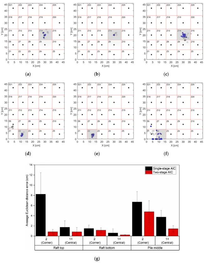
We applied the two-stage AIC picker to improve the accuracy in source localization. Figure 9 compares the source localization results of the two-stage AIC method against those of the single-stage AIC picker for the cases of Zones 2 and 14 as representatives of the corner and central zones. Table 1 also tabulate all the results of zonation accuracy and the average EDE. The results revealed
that the average EDE was reduced and the zonation accuracy was significantly improved in most of the cases. Both in the corner and central zones of RB cases and RT central case, there was a clear but small improvement after the application of two-stage AIC due to the sufficient accuracy with the single-stage AIC.
(a) (b) (c)
(d) (e) (f)
(g)
Figure 9. Localized sources estimated using the two-stage AIC method when the hit sources were on
a central and a corner region of the sensor network. Hits were applied on the raft top of Zone #14 (a) and #2 (d), under the raft bottom of Zone #14 (b) and #2 (e), and in the middle of Zone #14 (c) and #2 (f). The blue filled dot shows the result of two-stage AIC and the hollow gray dot shows the result of single-stage AIC. (g) The average Euclidian distance errors estimated from the single-stage and two-stage AIC methods.
By contrast, the greatest improvement in accuracy was achieved in the RT corner zones, in which the zonation accuracy was improved from 25% to 100% by using the two-stage AIC picker. Additionally, the average EDE was reduced from 8.24 cm to 0.87 cm. This significant improvement in accuracy at the RT corner zones can be explained by the large signal amplitude levels, which enables a two-stage AIC picker to distinguish between noise and signal and to increase the sensitivity of the AIC function value. The application of two-stage AIC reduced the average EDE from 6.72 cm to 4.81 cm in the PM corner zones, which is still considerably large with the lowest accuracy. This low accuracy is attributable to the low SNR of the signals in PM cases.
4. Discussion
4.1. Single-Stage AIC Method Versus Two-Stage AIC Method
Figure 10a–c compare the onset times determined by the single-stage AIC method for RT, RB, and PM cases. The onset times for RT and RB cases were well determined because the amplitude of the AE signals was large enough compared to the background noises. As a result, there was a clear valley with the minimum peak in the AIC curve, which estimated the first arrival of the AE signal well. Accordingly, this led to the average EDE of 2.65 cm for RT case and 1.08 cm for RB case.
(a) (b)
(c) (d)
Figure 10. The onset times estimated using the single-stage AIC method for the hit sources on the raft
top (a), under the bottom raft (b), and in the middle of the pile (c). The hit was located at Pile #14. Additionally, (d) the improved onset time estimated using the two-stage AIC method for the same hit in (c). The vertical (voltage) resolution in the 8-bit A/D converter was ~7.81 mV for the acquired signals in (a) and (b), and ~1.95 mV for the acquired signals in (c) and (d). The horizontal (time) interval was ~60 ns.
By contrast, the onset time in the PM case appears to be determined late compared to the actual onset time (Figure 10c). This caused a poor accuracy with the average EDE of 4.78 cm. It is due to the
combination of the low SNR up to the point of −150 μs and the abrupt increase in amplitude approximately at −50 μs, which flattened the AIC function near the minimum point (Figure 10c). In this study, we consistently found that the low SNR caused poor determination of the onset times by using the single-stage AIC picker, as the AE signal’s travel distance from the source to sensor increased.
Without any post-processing or filtering of signals, the onset time determination can be improved in the second-round AIC picker by using a narrower window that excludes the abrupt amplitude spikes [21]. Figure 10d shows the onset time determined by the two-stage AIC picker. Herein, the second round of the AIC used the window that included the minimum point of the 1st round AIC function and excluded the point of an abrupt increase in amplitude. As an example, for the PM case in Zone 2, the two-stage AIC picker more accurately localized the AE source with a decreased average EDE from 6.72 cm to 4.81 cm.
It appears that the single-stage AIC allows a sufficiently accurate estimation of the source location when a source is located at the raft top or raft bottom in the central zones. In such cases, the EDE was found to be less than 2.65 cm, equivalent to ~6% of the side length of the model PRF. By contrast, when a source is located in the RT-, RB-, and PM-corner zones or the PM-central zones, the application of the two-stage AIC is recommended to increase the accuracy.
4.2. Effect of Sensor Distance from the Source
It is widely conceived that the more sensors installed, the more information acquired, hence this leads to the higher accuracy in source localization. This is only valid when any of the acquired information is not false. By contrast, even though many sensors are installed, if one of them provides unclear information, it would interrupt data interpretation. Therefore, not only the information quantity but also the information quality is important. In real-time AE monitoring, filtering unclear information is as important as gathering more information from sensors.
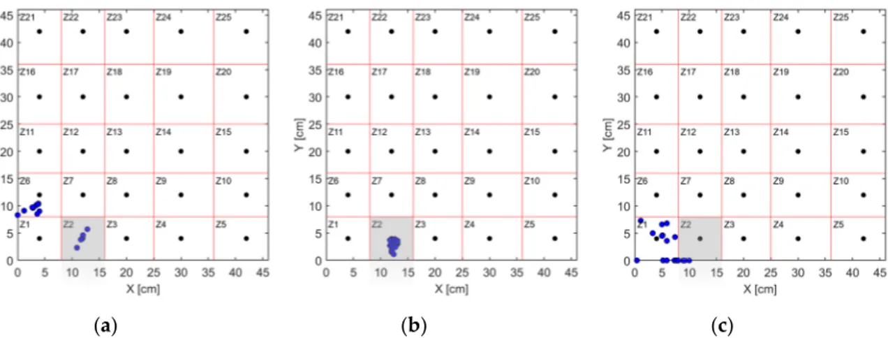
Meanwhile, AE signals attenuate fairly fast with increasing propagation distance due to the high-frequency characteristics. As an AE signal propagates through the model PRF, the signal becomes smoothed and its frequency range broadened evidently due to the various factors such as the frequency-dependent nature of scattering, geometric spreading, internal friction, mode conversion, and intrinsic attenuation in high-frequency content [8]. Additionally, the amplitude of a signal decreases rapidly, which results in a decrease in the signal-to-noise ratio (SNR). When the source location is distant from the AE sensor, the captured AE signal often shows low SNR, which prevents accurate determination of onset time. Expectedly, the source localization results for the PM cases in the corner zones show the high average EDE, compared to the central zones or the RT and RB cases, despite the use of the two-stage AIC method (Table 1). As an example, Figure 11 shows the onset times determined in all the accelerometers for the PM cases in Zone 2. In the two closest accelerometers ACC1 and ACC5, there was no difference in the onset times determined by single- and two-stage AIC pickers due to the large SNR. In the other accelerometers, there was the onset time difference in association with low SNR, owing to the long travel distance. There were some deviations between actual and estimated onset times in ACC3 and ACC4, which were the farthest accelerometers from the AE source. Therefore, the blind use of such inaccurate information can degrade the source localization.
Figure 11. The normalized waveforms generated at pile foundation of node #2 and estimated onset
time determined by 1st and 2nd AIC function at six different accelerometers. The onset times determined by the 1st and 2nd AIC function were marked with a black and red hollow dot. The amplitude of each signal was normalized with its peak amplitude for comparison.
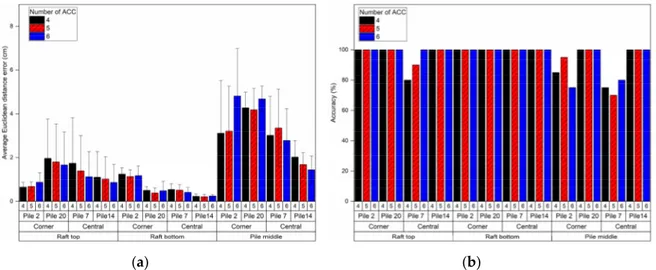
We examined if the exclusion of the onset times captured at the farthest two accelerometers would improve the accuracy in source localization. Herein, we computed the accuracy values while reducing the number of sensors from six to four. The accelerometers excluded changed, taking into account the source-to-sensor distance. For example, ACC 3 and ACC 4 were excluded for Zones 2 and 7. ACC 4 and ACC 5 were excluded for Zone 14. As a result, the accuracy increased when one or two farthest sensors were excluded for PM corner cases, as shown in Figure 12. However, the accuracy decreased when the sensors were excluded in most cases of RT and RB, which showed higher SNR when compared to the PM cases. This exercise confirms that filtering unclear information, particularly the signals captured at a far distance and with low SNR, can enhance the source localization accuracy.
(a) (b)
Figure 12. The accuracy improvement in source location by changing the number of sensors used for
5. Summary and Implication
This study proposes a real-time source localization using acoustic emission (AE) via scaled laboratory experiments. The algorithm, composed of the automatic single and two-stage AIC picker and Simplex method, was developed and its damage-source localization accuracy was examined with the signals generated at three different locations in the three-dimensional model scaled PRF: (1) raft top surface, (2) raft bottom surface, and (3) middle of a pile.
As a result, the automatic single-stage AIC picker showed poor prediction accuracy for the sources in RT corner zones and PM central zones, with less than 90% accuracy, although it fairly reliably predicted the source locations for those in RT and RB central zones and RB and PM corner zones, with the accuracy higher than 90%. By contrast, the two-stage AIC picker clearly showed better prediction capability, with an increase in the overall accuracy from 88.3% to 95.3% compared to the single-stage AIC picker. This result proves that the two-stage AIC picker can be a useful tool for the automatic determination of arrival time to locate AE events. In addition, some signals showed low SNR because of the long propagation path. In such cases, the exclusion of some signals with low SNR out of all collected signals can improve the accuracy of source localization, such as the ones detected from the farthest sensors.
For field implementation, the wave velocity of a structure of interest needs to be determined for accurate AE source location. The medium wave velocity used in the Simplex method has a significant influence on the accuracy in the source location. In our study, we found two cases: the RT and RB cases where the source is generated close to a raft versus the PM case where the source is generated in the middle of a pile. The use of P-wave velocity of the medium showed the best accuracy for the RT and RB cases, and using rod wave velocity resulted in good prediction accuracy for the PM case. Meanwhile, in PRF, the connection between the pile and the raft is the most prone to damage. Therefore, a source is most likely to occur close to the raft, though it is still uncertain and unknown at which location the crack or damage will be generated in foundations. In the field, it is suggested to measure the wave velocity, particularly the P-wave and rod wave velocities, on an exposed surface of the structure (e.g., concrete surface in a reinforced concrete structure). For example, the P-wave and S-wave velocities of reinforced concrete structures range ~3600–4200 m/s and ~2000–2500 m/s. We expect that the proposed approach exploiting the two-stage AIC picker to AE source localization can provide useful information on the damaged location in subsurface buried foundations that we cannot visually inspect.
In addition, the onset time determination by using an automatic AIC picker can be challenging in the field due to the ambient noises, such as rain, hail, and wind with debris [36]. The signal filtering has to be preceded to minimize the noise effect. Additionally, due to the rapid attenuation of signals, coverage area and detectable signal distance can be limited, and these depend on the type and array of sensors and source localization method.
Author Contributions: Conceptualization, H.K., M.O., J.-S.K., and H.K.; Methodology, Y.-M.K., H.K.,
T.-M.O., J.-S.K. and T.-H.K.; formal analysis, Y.-M.K.; investigation, Y.-M.K. and G.H.; data curation, Y.-M.K. and G.H.; writing—original draft preparation, Y.-M.K.; writing—review and editing, Y.-M.K., G.H., H.K., T.-H.K.; funding acquisition, H.K. T.-H.K.; all authors have read and agreed to the published version of the manuscript.
Funding: This research was supported by the Nuclear Research and Development Program of the National
Research Foundation of Korea (2020M2C9A1062949) funded by the Minister of Science and ICT, and by the National Research Council of Science & Technology (NST) grant by the Korea government (MSIP) (No. CRC-16-02-KICT).
Acknowledgments: We would like to thank three anonymous reviewers for providing valuable comments and
suggestions, which was very helpful to improve this manuscript.
References
1. Lockner, D. The role of acoustic emission in the study of rock fracture. Int. J. Rock. Mech. Min. 1993, 30, 883– 899.
2. Nair, A.; Cai, C.S. Acoustic emission monitoring of bridges: Review and case studies. Eng. Struct. 2010, 32, 1704–1714.
3. ASTM E1316. Standard Terminology for Nondestructive Examinations; ASTM international: West Conshohocken, PA, USA, 2006; pp. 1–33.
4. Grosse, C.U.; Finck, F. Quantitative evaluation of fracture processes in concrete using signal-based acoustic emission techniques. Cem. Concr. Compos. 2006, 28, 330–336.
5. Hensman, J.; Mills, R.; Pierce, S.G.; Worden, K.; Eaton, M. Locating acoustic emission sources in complex structures using Gaussian processes. Mech. Syst. Signal Process. 2010, 24, 211–223.
6. Holford, K.M.; Davies, A.W.; Pullin, R.; Carter, D.C. Damage location in steel bridges by acoustic emission.
J. Intell. Mater. Syst. Struct. 2001, 12, 567–576.
7. Kaphle, M.; Tan, A.C.; Thambiratnam, D.P.; Chan, T.H. Identification of acoustic emission wave modes for accurate source location in plate-like structures. Struct. Control Health 2012, 19, 187–198.
8. Oh, T.M.; Kim, M.K.; Lee, J.W.; Kim, H.; Kim, M.J. Experimental Investigation on Effective Distances of Acoustic Emission in Concrete Structures. Appl. Sci. 2020, 10, 6051.
9. ElBatanouny, M.K.; Ziehl, P.H.; Larosche, A.; Mangual, J.; Matta, F.; Nanni, A. Acoustic emission monitoring for assessment of prestressed concrete beams. Constr. Build. Mater. 2014, 58, 46–53.
10. Ohno, K.; Ohtsu, M. Crack classification in concrete based on acoustic emission. Constr. Build. Mater. 2010,
24, 2339–2346.
11. Ge, M. Efficient mine microseismic monitoring. Int. J. Coal Geol. 2005, 64, 44–56.
12. Han, Q.; Xu, J.; Carpinteri, A.; Lacidogna, G. Localization of acoustic emission sources in structural health monitoring of masonry bridge. Struct. Control Health 2015, 22, 314–329.
13. Hirata, A.; Kameoka, Y.; Hirano, T. Safety management based on detection of possible rock bursts by AE monitoring during tunnel excavation. Rock Mech. Rock Eng. 2007, 40, 563–576.
14. Carpinteri, A.; Xu, J.; Lacidogna, G.; Manuello, A. Reliable onset time determination and source location of acoustic emissions in concrete structures. Cem. Concr. Compos. 2012, 34, 529–537.
15. Pearson, M.R.; Eaton, M.; Featherston, C.; Pullin, R.; Holford, K. Improved acoustic emission source location during fatigue and impact events in metallic and composite structures. Struct. Control Health 2017,
16, 382–399.
16. Schechinger, B.; Vogel, T. Acoustic emission for monitoring a reinforced concrete beam subject to four-point-bending. Constr. Build. Mater. 2007, 21, 483–490.
17. Baer, M.; Kradolfer, U. An automatic phase picker for local and teleseismic events. B. Seismol. Soc. Am. 1987,
77, 1437–1445.
18. Hinkley, D.V. Inference about the change-point from cumulative sum tests. Biometrika 1971, 58, 509–523. 19. Maeda, N. A method for reading and checking phase times in auto-processing system of seismic wave data.
Zisin. 1985, 38, 365–379.
20. Eaton, M.; Pullin, R.; Holford, K. Toward improved damage location using acoustic emission. J. Mech. Eng.
Sci. Proc. Inst. Mech. Eng. Part C. 2012, 226, 2141–2153.
21. Zhang, H.; Thurber, C.; Rowe, C. Automatic P-wave arrival detection and picking with multiscale wavelet analysis for single-component recordings. Bull. Seismol. Soc. Am. 2003, 93, 1904–1912.
22. Mokhtar, I.; Yahya, M.Y.; Kadir, M.R.A.; Kambali, M.F. Effect on mechanical performance of UHMWPE/HDPE-blend reinforced with kenaf, basalt and hybrid kenaf/basalt fiber. Polym-Plast. Technol.
2013, 52, 1140–1146.
23. Sotomayor, M.E.; Krupa, I.; Várez, A.; Levenfeld, B. Thermal and mechanical characterization of injection moulded high density polyethylene/paraffin wax blends as phase change materials. Renew. Energy 2014,
68, 140–145.
24. Elshimi, T.M.; Moore, I.D. Modeling the effects of backfilling and soil compaction beside shallow buried pipes. J. Pipeline Syst. Eng. Pract. 2013, 4, 04013004.
25. ASTM E976, Guide for Determining the Reproducibility of Acoustic Emission Sensor Response; ASTM international: West Conshohocken, PA, USA, 2005.
26. Hsu, N.N.; Brecknbridge, F.R. Characterization and calibration of acoustic emission sensors. Mater. Eval.
27. Sause, M.G. Investigation of pencil-lead breaks as acoustic emission sources. J. Acoust. Emiss. 2011, 29, 184– 196.
28. Sikdar, S.; Ostachowicz, W.; Pal, J. Damage-induced acoustic emission source identification in an advanced sandwich composite structure. Compos. Struct. 2018, 202, 860–866.
29. Sikdar, S.; Mirgal, P.; Banerjee, S.; Ostachowicz, W. Damage-induced acoustic emission source monitoring in a honeycomb sandwich composite structure. Compos. Part B Eng. 2019, 158, 179–188.
30. Kurz, J.H.; Grosse, C.U.; Reinhardt, H.W. Strategies for reliable automatic onset time picking of acoustic emissions and of ultrasound signals in concrete. Ultrasonics 2005, 43, 538–546.
31. Mhamdi, L. Seismology-Based Approaches for the Quantitative Acoustic Emission Monitoring of Concrete Structures. Ph.D. Thesis, University of Delaware, Newark, DE, USA, 2015.
32. Sedlak, P.; Hirose, Y.; Khan, S.A.; Enoki, M.; Sikula, J. New automatic localization technique of acoustic emission signals in thin metal plates. Ultrasonics 2009, 49, 254–262.
33. Sedlak, P.; Hirose, Y.; Enoki, M. Acoustic emission localization in thin multi-layer plates using first-arrival determination. Mech. Syst. Signal Process. 2013, 36, 636–649.
34. Prugger, A.F.; Gendzwill, D.J. Microearthquake location: A nonlinear approach that makes use of a simplex stepping procedure. Bull. Seismol. Soc. Am. 1988, 78, 799–815.
35. Ge, M. Analysis of source location algorithms: Part II. Iterative methods. J. Acoust. Emiss. 2003, 21, 29–51. 36. Ziehl, P.; ElBatanouny, M. Acoustic emission monitoring for corrosion damage detection and classification.
In Corrosion of Steel in Concrete Structures; Woodhead Publishing: Cambridge, UK, 2016; pp. 193–209.
Publisher’s Note: MDPI stays neutral with regard to jurisdictional claims in published maps and institutional
affiliations.
© 2020 by the authors. Licensee MDPI, Basel, Switzerland. This article is an open access article distributed under the terms and conditions of the Creative Commons Attribution (CC BY) license (http://creativecommons.org/licenses/by/4.0/).