745
-Adaptive Detection of a Moving Target Undergoing Illumination Changes
against a Dynamic Background
Mu Lu1,2*, Yang Gao1, and Ming Zhu1,2
1Changchun Institute of Optics, Fine Mechanics and Physics, Chinese Academy of Sciences,
Changchun, Jilin 130033, China
2Key Laboratory of Airborne Optical Imaging and Measurement, Chinese Academy of Sciences,
Changchun, Jilin 130033, China
(Received August 11, 2016 : revised October 28, 2016 : accepted November 28, 2016)
A detection algorithm, based on the combined local-global (CLG) optical-flow model and Gaussian pyramid for a moving target appearing against a dynamic background, can compensate for the inadaptability of the classic Horn–Schunck algorithm to illumination changes and reduce the number of needed calculations. Incorporating the hypothesis of gradient conservation into the traditional CLG optical-flow model and combining structure and texture decomposition enable this algorithm to minimize the impact of illumination changes on optical-flow estimates. Further, calculating optical-flow with the Gaussian pyramid by layers and computing optical-flow at other points using an optical-flow iterative with higher gray-level points together reduce the number of calculations required to improve detection efficiency. Finally, this proposed method achieves the detection of a moving target against a dynamic background, according to the background motion vector determined by the displacement and magnitude of the optical-flow. Simulation results indicate that this algorithm, in comparison to the traditional Horn-Schunck optical-flow algorithm, accurately detects a moving target undergoing illumination changes against a dynamic background and simultaneously demonstrates a significant reduction in the number of computations needed to improve detection efficiency.
Keywords : Moving target detection, Combined local-global optical-flow model, Gaussian pyramid, Illumination changes
OCIS codes : (100.0100) Image processing; (100.2000) Digital image processing; (110.2970) Image detection systems; (330.4150) Motion detection
*Corresponding author: [email protected]
Color versions of one or more of the figures in this paper are available online.
*
This is an Open Access article distributed under the terms of the Creative Commons Attribution Non-Commercial License (http://creativecommons.org/ licenses/by-nc/3.0/) which permits unrestricted non-commercial use, distribution, and reproduction in any medium, provided the original work is properly cited.
*Copyright 2016 Optical Society of Korea I. INTRODUCTION
As research in the computer vision field advances, achieving progress in one of its most significant and widespread applications, dynamic background moving target detection, is imperative. The optical-flow method has proven to be essential for detecting and analyzing a moving target against a dynamic background [1, 2]. The optical-flow method possesses the advantages of high detection precision and the capacity to detect sheltered targets. Developed and refined over the course of 30 years, the optical-flow method is
widely applied in the field of image analysis. The concept of optical-flow was proposed by Gibson in 1950. In a video image, the grayscale of each pixel in the image is changed in time sequence, the relationship of the changes of each pixel can be used to determine the relative motion, thus detecting a moving target in the video image. The fundamental principle of the optical-flow method entails projecting each pixel in a video image sequence onto a three-dimensional (3D) object, assigning an equivalent velocity vector for each projection, and then processing a dynamic analysis of the 3D object using a velocity vector feature
[3-5]. The optical-flow field in a video frame is continuous when there is no relative movement between target and background; otherwise, it is discontinuous. Therefore, accessing continuous conditions of an optical-flow field in a video image enables detection of a moving target within that image.
Differential-based optical-flow and matching-based optical-flow algorithms are the most studied current optical-flow methods. The basic constraint equation rests on a differential optical-flow algorithm derived from the assumption of brightness constancy. According to differing constraint conditions, this paper presents two representative algorithms, the Horn-Schunck (HS) global optical-flow algorithm [6, 7] and the Lucas-Kanade (LK) local optical-flow algorithm [8, 9]. Based on the hypothesis of global smoothness, the HS global optical-flow algorithm computes the optical-flow of each point in a video image sequence [10]. Thus, the optical-flow acquired in this algorithm exhibits high density. In contrast, the LK algorithm, by assigning different weight values to the points in the neighborhood of the central point in a video image, computes the optical- flow at the central point using the weighted optical-flow of points in that neighborhood [11]. Thus, this algorithm requires a relatively sparse optical-flow. Based on matching algorithms [12, 13], optical-flow is defined by the displacement generated by a moving target fitting from different times. Typical methods calculate optical-flow by minimizing distance functions or maximizing cross-correlation functions [14].
In this paper, an improved combined local-global (CLG) optical-flow model used for moving targets in dynamic background detection is studied, this improved algorithm solves the problem that when applying a classic optical-flow algorithm to illuminate change condition, the optical-flow field is unreliable. Further combinations of the HS and LK optical-flow algorithms ensure the reduction of the amount of computation required to complete real-time detection of a moving target undergoing changing illumination against a dynamic background.
II. METHODS 2.1. Improved Optical-flow Algorithm
Optical-flow algorithms are well adapted to detect moving targets with moving cameras. These algorithms possess the advantages of using image information for calculations that do not need pre-processing or the ability to process sheltered targets. Two problems remain unsolved when applying the classic HS and LK optical-flow algorithms to practical applications. First, due to illumination changes, the hypothesis of brightness constancy is not applicable in certain areas. Thus, the optical-flow fields calculated in those areas are not reliable [15]. Second, classic algorithms, despite employing simple principles, require large amounts of computation and thus, cannot achieve real-time detection in some special circumstances [16].
2.2. Improvement to Adapt Illumination Change The classic HS optical-flow algorithm is based on the hypothesis of brightness constancy. The basic optical-flow constraint equation is 0 x y Iv Iv I x y t ∂ +∂ +∂ = ∂ ∂ ∂ , (1)
where vx and vy represent the optical-flow velocity in the
x- and y-directions, respectively. I denotes the grayscale image. According to the continuity and smoothness constraints of optical-flow, introducing the smoothness item i establishes the constraint equation
2
Ω[ ( ) ]
T T
HS
E =
∫
w ∇ ∇I I w+ ∇α w dxdy, (2) where w u v=[ , ,1]T. The HS optical-flow algorithm is easy to implement, but its stability and anti-noise performance are not satisfactory.Lucas, a contemporary of Horn, proposed a new optical- flow model based on the hypothesis of keeping the optical- flow velocity vector constant across a small area u. Thus,
( )
T T
LK
E =w Kρ• ∇ ∇I I w, (3)
where ρ is the standard deviation and Kρ is the Gaussian weight function. The LK optical-flow algorithm offers high stability but is not suitable for areas of images with small or no grayscale gradient.
To combine the advantages of the HS and LK optical- flow algorithms, Bruhn and his team proposed the CLG optical-flow model [17]:
2
[ T ( T) ]
CLG
E =
∫
Ω w Kρ ∇ ∇I I w+ ∇α w dxdy (4) Despite possessing the merits of both the HS and LK optical-flow algorithms, the CLG optical-flow model rests on the hypothesis of brightness constancy and, therefore, cannot adapt to illumination changes to achieve moving target detection.To solve this problem, an improved CLG optical-flow model is proposed. To reduce the sensitivity to illumination changes in this model, a new data term is adopted. This term is a combination of gradient conservation hypothesis and traditional CLG optical-flow model. Its energy equation is as follows: ( ) [ T ( T) T ( T x x E w =
∫
Ω w Kρ ∇ ∇I I w w K+ ρ ∇ ∇I I 2 ) ( )] T y y I I w αψ w dxdy + ∇ ∇ + ∇ , (5)where ψ(x) is the penalty function ψ( )s2 = s2+ε2 and ε is a positive minimum value. In this equation, ε is 0.0001.
Under the condition in which one conservation hypothesis is not valid, to ensure an acceptable result after performing computations, both grayscale conservation and gradient conservation are considered to yield an improved energy equation, where { [ T ( T) ] [ T ( T x x E=
∫
Ωψ w Kρ ∇ ∇I I w +ψ w Kρ ∇ ∇I I 2 ) ] } T y y I I w αψ w dxdy + ∇ ∇ + ∇ . (6)Restraining the effective illumination change enhances the performance of the algorithm; a structure and texture decomposition method is performed on video image sequences as a form of pre-processing. Input video image can be decomposed to texture information section IT and geometrical
information texture information section IS. Texture information
is barely affected by shadow, occlusion and luminous intensity change while geometrical information is vulnerable to those factors. The new input video image is defined as a linear combination of section IT and IS to adapt to
illumination change. In this case, =0.95
T S
I = −I αI α , (7)
where IT represents texture information of the video image,
IS represents the geometrical information of the video image.
I can be defined by x x y y t t x x xx xx yy yy xy xy xt xt yt yt I I I I I I I I I I I I I I I I I I = ∂ ⎧ ⎪ = ∂ ⎪ ⎪ = ∂ ⎪ = ∂ ⎪⎪ = ∂ ⎨ ⎪ = ∂ ⎪ = ∂ ⎪ ⎪ = ∂ ⎪ ⎪ = ∂ ⎩ . (8)
Then, treating Eq. (6) and Eq. (8) as a system of simultaneous equations produces 2 2 2 2 2 2 2 2 2 2 0 ( ) [ ( )] [ ( )] [ ( ) ] 0 ( ) [ ( )] [ ( )] [ ( ) ] t x t xt yt xx xt xy yt t y t xt yt yy yt xy xt K I K I I K I I K I I I I div u v u K I K I I K I I K I I I I div u v v ρ ρ ρ ρ ρ ρ ρ ρ ψ ψ α ψ ψ ψ α ψ ′ ′ ⎧ = + + ⋅ + − ⎪ ′ ⎪ ⋅ ∇ + ∇ ∇ ⎪ ⎨ ′ ′ = + + ⋅ + − ⎪ ⎪ ′ ⋅ ∇ + ∇ ∇ ⎪⎩ . (9)
According to the grayscale linear-invariance hypothesis, Eq. (9) is correct when u and v have sufficiently small values. In a practical target-detecting situation, because target displacement is relatively large, utilizing the method of fixed-point iterations to acquire the k-layer pyramid optical- flow increments duk and dvk can yield useful results. Thus
1 2 1 2 0 ( ) [ ( )] ( ) [ ( ) ( )] [( ) ( )] 0 ( ) [ ( )] ( ) [ ( k k k k k k k D x t x y k k k k k k k k k k k k k D xx xt xx xy xy yt xy yy k k k S k k k k k k k D y t x y k k k k k k D yy yt yx yy K I I I du I dv K I I I du I dv K I I I du I dv div u du K I I I du I dv K I I I du I dv ρ ρ ρ ρ ρ ψ ψ α ψ ψ ψ ′ = ⋅ + + + ′ ⋅ + + + + + − ′ ⋅ ⋅∇ + ′ = ⋅ + + + ′ ⋅ + + ) ( )] [( ) ( )] k k k k k k k xy xt xx xy k k k S K I I I du I dv div v dv ρ α ψ ⎧ ⎪ ⎪ ⎪ ⎪ ⎨ ⎪ ⎪ + + + − ⎪ ⎪ ⋅ ′ ⋅∇ + ⎩ , (10) in which 1 2 2 2 ( ) [ ( )] ( ) [ ( ) ( )] ( ) [ ( ) ( ) ] k k k k k k D t x y k k k k k k k k k k k D xt xx xy yt y xy k k k k k S K I I du I dv K I I du I dv I I du I dv u du v dv ρ ρ ψ ψ ψ ψ ψ ψ ⎧ ′ = ′ + + ⎪⎪ ′ = ′ + + + + + ⎨ ⎪ ′ = ′ ∇ + + ∇ + ⎪⎩ . (11) The improved CLG optical-flow algorithm solved the problem of low computing accuracy in optical-flow algorithms under conditions of changing illumination. It could not, however, achieve real-time moving target detection, because a certain number of iterations are required to meet the demand of high accuracy and such numbers of iterations need a large amount computation which consumes a long time. This study presents improvements aimed at reducing the needed amount of computation while simultaneously satisfying the system’s requirement of providing real-time detection. 2.3. Improvements to Reduce the Amount of Computation
To complete real-time moving target detection, the threshold segment method was adopted. In this method, the optical- flows of points whose grayscale gradient value was greater than the threshold were calculated using the improved CLG optical-flow algorithm in 2.2. Then, the optical-flows of other points were calculated by iterations. Next, the multi-layer Gaussian pyramid layered computational method was adopted and adjusted to the size of the image to reduce the amount of needed computation and to yield real-time detection.
The grayscale values of the pixel points generally remained the same after the target moved. This observation is approxi-mately true when considering large grayscale gradient points. Therefore, when applying the improved CLG optical-flow algorithm to large gradient points only, iterations of the algorithm to other points does not affect the accuracy of the algorithm.
TABLE 1. Comparison of computation times before and after implementing improved algorithm
Frame number Computation time for 100 iterations (ms)
Before using improved algorithm After using improved algorithm B&A algorithm
275 538 72 108 276 561 79 119 277 526 64 97 278 553 75 114 279 611 87 133 280 584 82 126 281 568 80 123 282 549 74 114
The weight function can be defined by
2 2 2 2 1 ( , ) 0 ω = ⎨⎧⎪ + > + ≤ ⎪⎩ x y x y I I T x y I I T , (12)
where T is the threshold. Correspondingly, Eq. (6) then can be changed to { [ψ ρ( ) ] ωψ[ ρ( Ω =
∫
T ∇ ∇ T + T ∇ ∇ T x x E w K I I w w K I I 2 ) ] αψ } + ∇ ∇ T + ∇ y y I I w w dxdy . (13)The optical-flow iteration formula for small grayscale points is ( ) ( ) ( ) ( 1) 2 2 2 ( ) ( ) ( ) ( 1) 2 2 2 k k k x y t k x x y k k k x y t k y x y I u I v I u u I I I I u I v I v v I I I
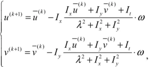
ω
λ
ω
λ
+ + ⎧ + + ⎪ = − ⋅ + + ⎪⎪ ⎨ ⎪ + + = − ⋅ ⎪ + + ⎪⎩ , (14)where λ is the weight coefficient which is set according to the precision requirement of derivatives, and are the local mean values of the optical-flow in the x- and y-directions, respectively.
Then, a Gaussian low-pass filter (GLPF) and image convolution method were adopted to process down-sampling two times to generate a three-layer Gaussian pyramid. For pixel points in the image, the bottom layer of the Gaussian pyramid was defined by g2 = 0. By practicing lift-sampling, the method then obtained the initial motion vector of the second layer of the Gaussian pyramid, where g1 = 2v2. Deducing from these results, the optical-flow of the top layer of the Gaussian pyramid is
3 0 ( , ) L L v x y d = =
∑
. (15)For low layers of the Gaussian pyramid, with fewer pixel points in an image, the optical-flow precision can be raised by increasing the number of iterations; for high layers of the Gaussian pyramid, the real-time performance of the algorithm can be improved by decreasing the number of iterations. Several frames of video images were selected and processed using the above-described algorithm. Table 1 summarizes a comparison of the computation times required for performing 100 iterations on eight separate video images both before and after implementing the improved algorithm. 2.4. Moving Targets in dynamic background detection
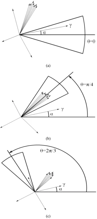
To detect the direction in which an image background is moving, a sliding window was established under polar coordinates to detect a moving vector based on the optical-flow calculated using the algorithm proposed in 2.3. The sliding window was fan-shaped, with a top angle of π/6. The position of the fan-shape was defined by the direction of the angular bisector of θ. In this arrangement, γ and α are the magnitude and direction of the motion vector, respectively. Then, m represents the number of motion vectors in the fan-shaped sliding window. This study utilized a 0.3-step-length forward-rotation fan-shaped sliding window and calculated the quantity of motion vectors in the fan- shaped sliding window. The sliding window enclosing the largest quantity of motion vectors was considered to be the computing result, as shown in Fig. 1.
Statistics characterizing the moving background vectors can be obtained from the amplitude of the motion vector
2 2 2 2 x y x y
v
v
v
δ
δ
δ
⎧ =
+
⎪
⎨
=
+
⎪⎩
, (16)(a)
(b)
(c)
FIG. 1. Directions of dynamic background motion estimations: (a) θ = 0, m = 1; (b) θ = π/4, m = 8; and (c) θ = 2π/3, m = 1.
where vx and vy are the mean values of the background motion vector in the x- and y-directions, respectively and δx
and δy are the deviations of the background motion vector in x- and y-directions, respectively. The amplitude of the motion vectors in the image appearing within the range of
1.7
v± δ can be considered as background. The general outline of the moving target can be acquired. After applying a morphological filter, a precision moving target area can
be determined, where , , 255 ( 1.7 ) ( , ) 255 ( 1.7 ) 0 others x y x y v v M x y v v δ δ ⎧ ≤ − ⎪⎪ =⎨ ≥ + ⎪ ⎪⎩ . (17)
III. RESULTS AND DISCUSSION
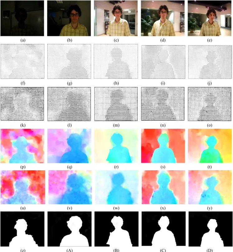
To test the validity of the algorithm designed to detect a moving target undergoing changes in illumination against a dynamic background, we utilized a computer with 2GB of memory and an Intel Pentium 2.60 GHz processor to complete MATLAB simulation experiments. The images in Fig. 2 depict the results of video detection performed on David, the subject. The video included 770 frames; each frame was 320 × 240 pixels.
In contrast to the HS optical-flow algorithm, the B&A brightness constancy model adapts to illumination change, provides a better experimental result, thus is used as a comparison with algorithm proposed in this paper. Figure 2 illustrates that under dramatic illumination changes, this improved algorithm can generate optical-flow fields and optical-flow vectors to distinguish the moving target more clearly. It also can maintain the optical-flow in the same direction as the moving target. Thus, the problem posed by the inability of the traditional optical-flow algorithm to adapt to illumination changes is solved in this study. The improved algorithm achieves high-precision detection of a target undergoing illumination changes and moving against a dynamic background.
To verify further the effectiveness of this algorithm, comparison experiments of this and another algorithm are practiced using an ECSSD (Extended Complex Scene Streams Dataset) standard database. PR curves of these algorithms are shown in Fig. 3. It can be seen that this algorithm showed higher accuracy and recall rate.
IV. CONCLUSION
This paper presents an improved CLG optical-flow model combining the Gaussian pyramid and structure and texture decomposition methods. In contrast to the classic optical- flow algorithm, this improved algorithm adapts to illumination changes, reduces the amount of required computation, and performs real-time detection. To satisfy the requirements for making practical use of real-time detection, this algorithm utilizes a combination of a Gaussian low-pass filter and an image convolution method, decreasing the average time consumed to perform 100 iterations from 561.2 ms to 76.6 ms. Simulation experiments show that the optical-flow algorithm proposed in this study completes high-precision moving-
(a) (b) (c) (d) (e) (f) (g) (h) (i) (j) (k) (l) (m) (n) (o) (p) (q) (r) (s) (t) (u) (v) (w) (x) (y) (z) (A) (B) (C) (D)
FIG. 2. Source frames, related optical-flow figures, and results of moving target detection: (a) Frame number 14; (b) Frame number 276; (c) Frame number 518; (d) Frame number 576; (e) Frame number 671; (f)~(j) Optical-flow vector figure using algorithm in this paper; (k)~(o) Optical-flow vector figure using B&A brightness constancy algorithm; (p)~(t) Optical-flow field figure using algorithm in this paper; (u)~(y) Optical-flow field figure using B&A brightness constancy algorithm; (z)~(D) Result of moving target detection using algorithm in this paper.
target detection in conditions with changing illumination and dynamic backgrounds and performs real-time detection,
thus satisfying the practical demands for engineering appli-cations.
REFERENCES
1. W. Hu, T. Tan, and S. Maybank, “A Survey on Visual Surveillance of Object Motion and Behaviors,” IEEE Trans. Syst., Man, Cybern., Syst., Part C (Applications and Reviews), 34(3), 334-352 (2014).
2. K. Zhang, L. Zhang, and M. H. Yang, “Real-Time Com-pressive Tracking,” in Proc. 12th European conference on Computer Vision (Florence, Italy, Oct. 2012), pp. 864-877. 3. M. H. Jeong, “Image Blurring Estimation and Calibration with a Joint Transform Correlator,” J. Opt. Soc. Korea 18(5), 472-476 (2014).
4. Y. Wei, F. Wen, W. Zhu, and J. Sun, “Geodesic Saliency Using Background Priors,” in Proc. 12th European conference on Computer Vision (Florence, Italy, Oct. 2012), pp. 29-42. 5. Y. Feng, R. H. Zhang, L. S. Zhang, H. W. Wu, and J. M.
Xia, “Lane Detection Algorithm for Night-time Digital Image Based on Distribution Feature of Boundary Pixels,” J. Opt. Soc. Korea, 17(2):188-199 (2013).
6. P. Sundberg, T. Brox, M. Maire, P. Arbelaez, and J. Malik, “Occlusion boundary detection and figure/ground assignment from optical flow,” IEEE Conference on Computer Vision and Pattern Recognition 2011, (Crowne Plaza, Colorado, USA, Jun. 2011), pp. 2233-2240.
7. M. Heikkila and M. Pietikainen, “A texture-based method for modeling the background and detecting moving objects,” IEEE Trans. Pattern Anal. Mach. Intell. 28(4), 657-662 (2006). 8. Z. Jiang and L. H. Ding, “Aerial video image object
detection and tracing based on motion vector compensation and statistic analysis,” In Proc 2009 IEEE Asia Pacific Conference on Postgraduate Research in Microelectronics and Electronics (Shanghai, China, Nov. 2009), pp. 302-305.
9. B. H. Do and S. C. Huang, “Dynamic background modeling based on radial basis function neural networks for moving object detection,” In Proc 2011 IEEE International Conference on Multimedia and Expo, (Barcelona, Spain, Jul. 2011), pp. 1-4.
10. W. H. Lee, “Foreground objects detection using multiple difference images,” Opt. Eng. 49(4), 047201 (2010). 11. S. Vladimir and K. K. Sung, “Reference Functions for
Synthesis and Analysis of Multiview and Integral Images,” J. Opt. Soc. Korea 17(2), 148-161 (2013).
12. Y. Yang, M. Fu, X. Yang, G. Xiong, and J. Gong, “Auto-nomous ground vehicle navigation method in complex environment,” 2010 IEEE Intelligent Vehicles Symposium, (San Diego, CA, USA, Jun. 2010), pp. 458-460.
13. T. Liu, J. Sun, N. N. Zheng, X. Tang, and H. Y. Shum, “Learning to Detect a Salient Object,” In Proc 2007 IEEE Conference on Computer Vision and Pattern Recognition, (Minneapolis, MN, USA, Jun. 2007), pp. 1-8.
14. T. Meier and K. Ngan, “Automatic segmentation of moving objects for video object plane generation,” IEEE Trans. Circuits Syst. Video Technol. 8(5), 525-538 (1998).
15. S. Baker, D. Scharstein, J. Lewis, S. Roth, M. Black, and R. Szeliski, “A Database and Evaluation Methodology for Optical Flow,” Int. J. Comput. Vision 92(1), 1-31 (2010). 16. S. Sun, D. Haynor, and Y. Kim, “Motion estimation based on optical flow with adaptive gradients,” In Proc. 2000 International Conference on Image Processing, (Vancouver, Canada, Sept. 2000), pp. 852-855.
17. B. Andres, W. Joachim, F. Christian, K. Timo, and S. Christoph, “Real-Time Optic Flow Computation with Variational Methods,” Computer Analysis of Images and Patterns, (Springer Berlin Heidelberg, Germany, 2003), pp. 222-229