ARTICLE
International Journal of Advanced Robotic Systems
Three-dimensional Sound Source
Localization Using Inter-channel Time
Difference Trajectory
Regular Paper
Sangmoon Lee
1*, Youngjin Park
1and Youn-sik Park
11 KAIST, Daejeon, Republic of Korea
*Corresponding author(s) E-mail: [email protected] Received 04 July 2013; Accepted 28 September 2015 DOI: 10.5772/61652
© 2015 Author(s). Licensee InTech. This is an open access article distributed under the terms of the Creative Commons Attribution License (http://creativecommons.org/licenses/by/3.0), which permits unrestricted use, distribution, and reproduction in any medium, provided the original work is properly cited.
Abstract
Sound source localization is one of the basic and essential techniques for intelligent robots in terms of human-robot interaction and has been utilized in various engineering fields. This paper suggests a new localization method using an inter-channel time difference trajectory, which is a new localization cue for efficient 3-D localization. As one of the ways to realize the proposed cue, a two-channel rotating array is employed. Two microphones are attached on the left and right sides of the spherical head. One microphone is in a circular motion on the right side, while the other is fixed on the left side. According to the rotating motion of the array, the (source) direction-dependent characteristics of the trajectories are analysed using the Ray-Tracing formula extended for 3-D models. In simulation, the synthesized signals generated by the fixed and rotating microphone signal models were used as the output signals of the two microphones. The simulation showed that the localization performance is strongly dependent on the azimuthal position of a source, which is caused by the asymmetry of the trajectory amplitude. Additionally, the experimental results of the two experiments carried out in the room environment demonstrated that the proposed system can localize a Gaussian noise source and a voice source in 3-D space.
Keywords Three-dimensional Sound Source Localization, Inter-channel Time Difference Trajectory, Rotating Micro‐ phone Array, Ray-tracing Formula, Human-Robot Interac‐ tion
1. Introduction
Recently, intelligent robots have been developed to not only support arduous human tasks, but also to interact with people in order to meet various human needs [1, 2]. As an independent object with its own intelligence [3], a robot needs to recognize environmental changes, such as the appearance of unidentified objects or the acoustic events for missions completed. For example, robots working in households should detect user voices and simultaneously be aware of other acoustic events, such as noises emitted from home appliances and other voices from electric devices. As a result, they can pay attention to speakers with more natural human-robot interaction (HRI) skills. In this situation, the technology of sound source localization (SSL) is employed to estimate the acoustic source direction using the acoustic signals from the microphone array; this is one of the most important building blocks of HRI. In addition,
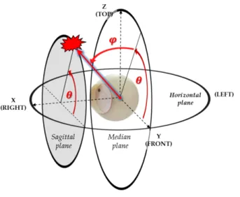
intelligent robots need to estimate the azimuth and elevation angles of a source together (i.e., 3-D SSL), due to the fact that a sound event occurs at an arbitrary direction in 3-D space. It is noteworthy, however, that a lot of techniques need to be carried out simultaneously with the given limited resources and the computational power for SSL is restricted. As a result, the computationally efficient 3-D SSL method is increasingly required. In addition, the source direction is defined by the inter-aural polar coordi‐ nates shown in Figure 1.
In the last few decades, many different SSL algorithms that are applicable to intelligent robots [4, 5] and also other engineering systems (e.g., teleconference systems [6] and surveillance units [7]) have been proposed. Even if the microphone array size, shape and number of microphones differ due to the constraints of various applications, certain localization cues (or direction estimation cues) are com‐ monly used: channel time difference (ICTD), inter-channel level difference (ICLD) and inter-inter-channel spectral difference (ICSD). ICTD is defined as the time difference between the arrivals of a sound wave-front to the micro‐ phones; ICLD is defined as the difference between the sound pressure levels at the microphones; and ICSD means the difference between the spectral contents at the micro‐ phones. ICTD has been used as the most powerful locali‐ zation cue [8-10] in almost all applications. Comparatively, ICLD and ICSD have not been used as frequently for practical applications, but are nevertheless employed in biomimetic research, including that of ear-based SSL systems [11, 12].
Figure 1. A sound source direction is defined in the inter-aural polar
coordinates by both the azimuthal angle (φS) and the elevation angle (θS).
The sagittal plane is a vertical plane dividing the space into right and left halves. Sources on each sagittal plane share the same azimuth. The median plane is the mid-sagittal plane that bisects the space symmetrically from left to right. The horizontal plane is perpendicular to the sagittal plane and passes through the centre of the coordinates.
In general, most of the SSL systems use more than four microphones for 3-D SSL. Except for circumstances in which directional microphones are used, if only two microphones are used and their locations do not change with time, 3-D SSL is not possible, because front-back confusion occurs due to the existence of many directions sharing the same localization cues, even for a single SSL [13, 14]. This is called the cone-of-confusion in 3-D space. In the absence of an additional structure (e.g., a spiral-shaped structure), more than four microphones in different (imaginable) planes are necessary in order to solve the cone-of-confusion problem inherent to 3-D SSL [15]. However, in the situation where a two-channel moving array for 3-D SSL is used, the measured localization cue such as ICTD will change according to the array motion. Then, from the changing pattern of ICTDs, it is expected that 3-D SSL can be achievable. Therefore, the (microphone) position-dependent ICTDs can be represented as below:
(
S, S)
t j q a (1)
where α is the parameter that identifies the location or the motion of the moving microphone. Here, the (source) direction- and (microphone) position-dependent ICTDs are named as the ICTD trajectory, which is the new concept for a localization cue for efficient 3-D SSL.
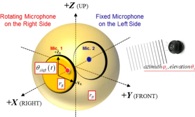
This paper proposes a 3-D SSL method using the ICTD trajectory induced by the circular motion of the two-channel rotating array. This array was selected as one of the possible ways to realize a specific ICTD trajectory. One of the two microphones is attached to the rotating plate on the right side of the spherical head, indicated by the red-coloured circle in Figure 2; the other microphone is fixed on the left side of the head, indicated by the blue-coloured circle. Figure 2 shows the schematic drawing of the suggested two-channel rotating microphone array instal‐ led on the spherical head. In this paper, in order to generate the known movement of the array, the circular motion is given to the right-sided plate.
This paper is organized as follows: in section 2, we intro‐ duce the new specific localization cue that is the ICTD trajectory relevant to the circular motion of the array. The mathematical derivation of the ICTD trajectory is presented using the extended Ray-Tracing formula for 3-D models. The relationship between the parameters of the ICTD trajectory and the source direction is also presented. Section 3 describes the proposed 3-D SSL algorithm based on the source direction estimator. In section 4, the localization performance of the proposed SSL algorithm is examined using simulations: the signal models of both rotating and fixed microphones are presented. Section 5 shows the experimental setup and the results using two kinds of sources. The discussion is presented in section 6 and the concluding remarks are given in section 7.
Figure 2. Schematic of the rotating microphone array installed on the
spherical head. One of two microphones is attached to the rotating plate on the right side of the head (red-coloured circle). In this paper we call this component the “rotating microphone”. The rotating part is moving in a clockwise direction on theYRZR plane and the shift angle of this part is measured with respect to the +ZR axis. The other microphone is fixed on the left side of the head (blue-coloured circle). It is called the “fixed micro‐ phone”.
2. Localization Cue: ICTD Trajectory
Most of the conventional localization algorithms have been developed using a microphone array fixed at given positions [4, 5, 8-12, 15] and with constant direction-dependent cues, on the assumption that a source position does not vary. The most commonly used time delay estimation (TDE) method is to use the generalized cross-correlation (GCC) function, which is employed to estimate ICTD between the selected pair of micro‐ phones [16, 17]. Among various GCC functions, the GCC-phase transform (PHAT) function is widely used because it is well known for its robust estimations of ICTD in the reverberant field [18].
If we use N omnidirectional microphones, N(N-1)/2 GCC-PHAT functions are obtainable. The GCC-GCC-PHAT function between the ith and jth microphones is defined as below [16]:
( )
( )
( )
2 i j i j i j x x j f x x x x G f R e df G f p t t ¥ -¥ =ò
(2)where f is the frequency and τ is a time delay variable. xi
and xj are defined as the ith and jth microphone output signals. Gxixj and Rxixj are the cross-spectral density function and the GCC-PHAT function between xi and xj, respective‐ ly. The τij, the measured ICTD between xi and xj, is calcu‐ lated by τij=argmaxτRxixj(τ). After that, the estimated direction of the sound source can be found by the relation‐ ship between the geometry of the microphone array and the multiple ICTDs. For example, when two microphones are placed on the horizontal plane and apart from each other by L m, the azimuth of a source can be estimated by using equation (3) [19]: $ cos1 12 S cL t j = - æ × ö ç ÷ è ø (3)
where c is the speed of sound and φ^S is the estimated azimuth. For example, SSL using ICTD maps [20, 21] was applied to the microphone array fixed on the robot head.
2.1 ICTD Trajectory
When using an immovable microphone array, the obser‐ vation of the constant localization cues (e.g., the ICTDs) can be used to efficiently estimate a direction, provided there are sufficient sensors. However, like the two-channel array, the measurement of the single constant localization cue does not guarantee successful SSL due to the cone-of-confusion problem. Thus, it is concluded that the useful 3-D SSL cue should have other characteristics dependent on the source direction, i.e., azimuth and elevation angles. When using the two-channel rotating array, if the angular velocity is given as wR, the position-dependent ICTD must be a periodic function with a period of 2π
/
wR. It is also noteworthy that the localization cue we want to suggest is similarly based on the ICTD concept. We assumed that the Doppler effect caused by the relative motion between the rotating microphone and a source can be ignored, because the speed of the rotating microphone, i.e., the radius of the rotating circle multiplied by the rotating angular speed is quite small compared with the speed of sound. Further‐ more, when considering the application scenario where the talking person as a target source is walking inside a room, the sound source is supposed to move slowly. Thus, the new specific localization cue, including the position-dependent feature of the circular motion of the rotating array, is defined in equation (4) for the source at (φS, θS):(
S, S Shift)
t j q q (4)
where θshift∈ 0, 2π and is measured clockwise from the
+ZR axis. Also, θshift indicates the position of the microphone
on the right side given a constant rotating radius (rR).
2.2 Extended Ray-Tracing Formula for 3-D Models
The well-known Ray-Tracing formula [22, 23] has been widely used for 2-D models to approximate the inter-aural time difference. However, in order to achieve the ICTD trajectories, this formula should be extended for 3-D models such as a two-channel rotating array installed on the sphere. Figure 3 shows the nomenclatures required to model the propagation distance between the source and the sensor locations. Once the propagation distance is derived, depending on the shift angle of the rotating part, the ICTD trajectory is obtainable with the assumption that the speed of the sound is independent of frequency in a non-disper‐
sive medium. In order to derive the propagation distance, three direction vectors fromCH to the positions of the two
microphones and the source need to be expressed as a function of the shift angle and the source direction.
(
rHcos , sinqR Rr qshift R, cosr qshift)
= uur R d (5)
(
rH,0,0)
= -uur F d (6)(
sin ,cos cos ,cos sin)
S=rS jS jS qS jS qS uur d (7) where dR → and dF →
are the direction vectors fromCH to the
rotating and fixed microphones respectively, rS is the distance between a source and CH, and dS
→
is the direction vector from CH to the source.
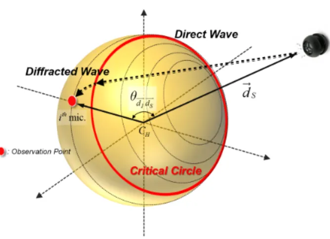
The Ray-Tracing formula for the 3-D model includes the concept of the critical circle, which is the counterpart of the critical point in the 2-D model [22]. When the observation point is hidden by the head, the wave-front from the source initially propagates to the critical circle directly and then secondarily propagates along the surface to the observation point. These propagation steps are shown in Figure 4 and the critical circle is represented by the red-coloured line. If we denote the direction vector to the ith microphone on the
surface as d→I, then the angle between two direction vectors (i.e., d→I and d→S) is denoted as θd→I
ds
→ and defined below:
1 cos I S I S d d I S d d d d q = - æç × ö÷ ç ÷ ç ÷ è ø uuruur uur uur uur uur (8)
Figure 3. Nomenclatures related to the rotating microphone array on the
spherical head. The centre of the head (CH) is at the origin of the XYZ coordinates. The red circle represents the rotating microphone at the rotating part on the YRZR plane. This microphone is rotating with a constant speed
(rR×wR), where rR and wR are the rotating radius and angular velocity, respectively. `The rotation centre CR is located at ( rH2−rR2, 0, 0). The shift
angle (θshift) of the rotating plate is defined as the angle from the + ZR axis
in a clockwise direction. The blue circle represents the fixed microphone that is located at (−rH, 0, 0). rH is the radius of the spherical head and θR is the
angle between the X axis and the direction vector to the rotating microphone from CH.
Figure 4. Two steps of wave propagation from the sound source to the
hidden observation point are illustrated by the green and purple lines. If the observation point (indicated by the red point) is hidden by the sphere from the view of the source, the wave-front approaches the critical circle directly. After that, the wave-front reaches the observation point along the surface.
Then, θd→Rd→s and θd→Fd→s can be expressed by equations (9) and (10) with the assumption that rS≫rH :
(
)
1shift
shift shift
cos (cos sin sin cos cos sin sin cos sin cos )
R S R S d d R S R R S S q q q j q j q q q j q q -= + + uuuruur (9) 2 F S S d d p quuuruur= +j (10) If θdR → ds →≤θ
c where θc is cos−1
(|
d→R| / |
d→S|)
~90o, then the wave propagates along the direct path only. Otherwise, if the microphone is hidden by the spherical head, which mathematically indicates that θd→Rd→s≥θc, the propagation distance by the diffracted wave motion along the surface should also be considered. Here, equation (11) shows the propagation distance from the source to the rotating microphone, denoted by DR, and equation (12) shows the distance from the source to the fixed microphone, repre‐ sented by DF :( )
( )
(
)
2 2 2 cos , sin , R S R S R S R S S H S H d d d d c R S c H d d c c d d r r r r D r r q q q q q q q q p ì + - £ ï = í ï + - £ £ î uuuruur uuuruur uuuruur uuuruur (11)( )
( )
(
)
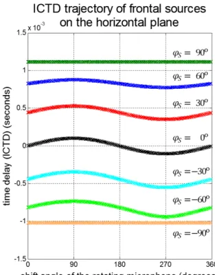
2 2 2 cos , sin , F S F S F S F S S H S H d d d d c F S c H d d c c d d r r r r D r r q q q q q q q q p ì + - £ ï = í ï + - £ £ î uuuruur uuuruur uuuruur uuuruur (12) If we denote Dd∞ as lim rs→∞DF− DR, the ICTD trajectories can be obtained by dividing Dd∞ by c. For example, when the physical dimensions of the rotating microphone array are those given in Table 1, the resulting ICTD trajectories of the
frontal sources on the horizontal plane are those shown in Figure 5. It is clear that the mean of the ICTD trajectories varies according to the change in the azimuth angle of the source, because theYRZR plane, on which the circular
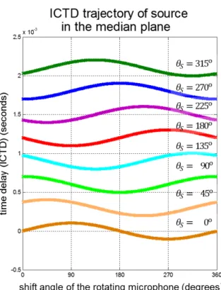
motion of the rotating microphone occurs, is perpendicular to the X axis. Also, for the frontal sources, the resulting up-and-down pattern of the ICTD trajectories is expected because of the clockwise microphone motion from the +ZR axis. On the other hand, we can conjecture that the pattern of the ICTD trajectories of the rear sources will be reversed. In addition, for the laterally biased sources, no significant features are visible because the source is on the X axis, which is the symmetric axis of the array’s rotating motion. Figure 6 shows the ICTD trajectories for the sources on the median plane. The vertical axis has no physical meaning because we added a 0.3 ms offset to the original ICTD trajectories as the elevation angle of the source increases by 45°, in order to present all ICTD trajectories in a single graph. As shown in Figure 6, as the elevation angle is increased, the phase of the trajectory is shifted. The source elevation angle is defined on the sagittal plane and the shift angle of the rotating part is also defined on the sagittal plane, i.e., the YRZR plane; see Figures 1 and 3. This is why the ICTD trajectory is shifted as much as the change of the elevation angle of a source. Then, it seems possible to estimate a source’s elevation angle by finding the phase shift of the trajectory. Therefore, we can expect that the mean value of the ICTD trajectories will be a useful cue for the azimuth estimation and an amount of the shift of the ICTD trajectory can be used to efficiently estimate the elevation.
Nomenclatures Numerical Values
rS 10 m rR 3.5 cm rH 15 cm wR= dθshift/dt 600 rpm. θR 0.236 rad. CR (0.146 m, 0 m, 0 m) CH (0 m,0 m, 0 m)
Table 1. The dimensions of the rotating microphone array and the angular
speed of the rotating part are given
2.3 Characteristics of the ICTD Trajectory of the Rotating Microphone Array
In section 2.2, examples of the ICTD trajectories obtained using the Ray-Tracing formula were shown. In section 2.3, we describe the characteristics of the ICTD trajectories of the rotating microphone array. First, the relation between the mean of the ICTD trajectory and the azimuth angle of the source will be derived. Second, the relation between the phase shift of the trajectory and the elevation angle will be
shown. In addition, the amplitude of the ICTD trajectory will be presented as a function of the azimuth angle only. First of all, the mean value of the ICTD trajectory is defined as equation (13):
(
)
2 shift shift 0 1 ICTDT= 2 c Dd d p q q p ¥ò
(13)The wave propagation from a source to a microphone is strongly dependent on the azimuth angle of a source; see Figure 4 and equation (10). For example, when a sound source is to the left of the head, only direct wave propaga‐ tion occurs to the fixed microphone. On the other hand, the consecutive propagation along the direct and indirect paths occurs from the source to the rotating microphone because the rotating microphone is hidden by the head from the view of the source. If a source is to the right of the head, the wave propagation characteristics are reversed. In particu‐ lar for a source with an azimuth angle within −θR, + θR, the propagation characteristic to the rotating microphone changes according to its shift angle. In order to represent propagation characteristics more precisely, we divide them into three categories: (case 1) the wave propagation is along the direct path only, (case 2) the Figure 5. The ICTD trajectories of the frontal sources on the horizontal plane.
The up-and-down motion of the ICTD trajectories is apparent because the shift angle of the rotating microphone increases in a clockwise direction from the +ZR axis. Additionally, for the left- and right-sided sources, the ICTD
trajectories described by the cyan dotted lines have no significant features because the propagation from the laterally-biased source to the rotating microphone does not change as the shift angle varies.
consecutive propagation is along the direct and indirect paths and (case 3) There is a transition between case 1 and case 2, depending on the shift angle. In terms of these categories, Table 2 shows the propagation characteristics according to the azimuth angle of the source. For the sources with azimuth angles within −θR, 0, the propa‐ gation to the rotating microphone corresponds to case 3. The transition from case 1 to case 2 occurs when the rotating microphone passes θb and the subsequent transition from case 2 to case 1 occurs at π + θb, where θb is defined in equation (14). For the sources with azimuth angles within 0, + θR , the transition from case 1 to case 2 occurs at θb and the consecutive transition from case 2 to case 1 occurs at π −θb :
( )
minarg sin tan cot
shift
b shift S R
q
q = é q £ j q ù
ë û (14)
where θshift∈ 0, 2π. With respect to the azimuth interval,
the mean value of the ICTD trajectory is derived as a function of the azimuth angle of the source only as shown in Figure 7. It is apparent that a one-to-one relationship exists between the mean value of the ICTD trajectory and the azimuth angle of the source. Therefore, it is possible to estimate the azimuth angle of the source once the mean value of the ICTD trajectory is obtained.
Figure 6. The ICTD trajectories for sources on the median plane are shown.
As the source elevation changes, the trajectory pattern shifts. For the source on the top of the head, the distance between the rotating microphone and the source is the shortest at θshift= 0°, which indicates that the ICTD is
maximal. The distance increases up to θshift= 180° and goes back to the shortest distance within a single period.
The Azimuth Intervals Corresponding Microphone Fixed Mic. Rotating Mic.
− π/2, − θR Case 1 Case 2
− θR, 0 Case 1 Case 3
0, + θR Case 2 Case 3
+θR, π/2 Case 2 Case 1
Table 2. The wave propagation characteristics from the source to the rotating
and fixed microphones
Figure 7. The mean value of the ICTD trajectory as a function of the azimuth
angle only is shown. The one-to-one relationship between the mean value of the ICTD trajectory and the azimuth angle is clearly defined. The vertical dashed lines indicate the azimuth angles (i.e., ±θR. θR is cos−1
(
rH2−rR2/
rH)
=13.4934°) in the rotating microphone array with dimensions as in Table 1.
On the other hand, the specific shift angles, which corre‐ spond to the maximal or minimal values of the ICTD trajectory, are useful for finding the elevation angle of the source. These specific shift angles are defined as below:
(
)
(
)
shift shift max shift shift min shift shift arg max arg min d d D D q q q q q q ¥ ¥ = = (15)which implies that θshiftmax and θshiftmin are equal to π
/
2−θS and 3π/
2−θS, respectively. It is obvious that the elevation angle increases from the +Y axis in an anticlockwise direction, while the shift angle of the rotating microphone increases from the +ZR axis in a clockwise direction (see Figures 1 and3). In summary, by finding the two parameters of the ICTD trajectory, i.e., ICTDT¯ and θshiftmax/min, the azimuth and elevation angles of the source can be found independently. In addition, as shown in Figure 5, the amplitude of the ICTD trajectory changes as the azimuth angle is varied. Natural‐ ly, we can expect the trajectory amplitude to be dependent on the azimuth angle only. Its definition is given below:
( )
max( )
minshift shift
1
ICTDT =PP c Dd¥ q -Dd¥ q (16)
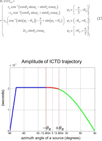
We express the amplitude of the ICTD trajectory as its peak-to-peak value using the specific shift angles in equation (15). Figure 8 visualizes its amplitude as a function of the azimuth angle. It is notable that the ICTD trajectories of the left-sided sources have larger ICTDTpp compared with those of the right-sided sources, except the source at
(
φS, θS)
= (−90°, 0°). The variation of the ICTD trajectory is affected due to the motion of the rotating microphone only. When the sphere hides the entire trajectory of the rotating microphone’s motion from the view of the source, the wave propagation in case 2 occurs, and the variation of the propagation distances becomes the largest (see Table 2). Also, when the source moves from the left to the right, the portion of the direct wave propagation increases and the ICTDTpp decreases. Equation (17) shows the ICTDTpp according to azimuth intervals:(
)
(
)
(
)
(
)
(
)
1 1 1 ICTDT =cos cos sin sin cos
, 2 cos cos sin sin cos
= cos sin sin ,
2 2 sin cos , 2 PP H R S R S S R H R S R S H S R S R S R R H R S S R r r r r q j q j j p q q j q j p j q j q j q q p q j j q -ì - é ùü ï Î -ê - úï - + ï ë ûï ï ï æ ö ï - - + + Î -é + ùï í çè ÷ø ë ûý ï ï ï é ùï Î + + ï ê úï ï ë ûï î þ (17)
Figure 8. The values of ICTDTpp are a function of the azimuth angle. In
particular, the left-sided sources within −π/2 + θR, −θR have the same
ICTDTpp, which corresponds to the time taken for a wave-front to travel the
length of 2rRθR, and 2rRθR/c is equal to 0.206 msec. 2rRθR is the greatest length made by the rotating motion on the surface within a full revolution. As a source approaches the right, ICTDTpp decreases. Exceptionally, the
ICTDTpps of the sources at (-90°, 0°) and (+90°, 0°) are zero, because these
sources are located on the X axis, which is perpendicular to the YRZR plane.
3. Localization Algorithm
The localization of a source can be achieved using the one-to-one relationship between the parameters of an ICTD trajectory and a source direction, as described in section 2.3. However, it is not easy to apply this approach to a real situation where a source and other noises are present simultaneously. In addition, the duration of a source varies and can be too short to calculate τ
(
θshift)
, even for a singlesource case. Therefore, to apply the practically feasible SSL to a real environment, a new SSL method is necessary. Section 3.1 presents the source direction estimator (SDE) based on the ICTD trajectory and section 3.2 summarizes the proposed 3-D SSL algorithm.
3.1 Source Direction Estimator
As mentioned before, we used the conventional GCC-PHAT function [16] to obtain the ICTD trajectories. Equation (18) redefines a GCC-PHAT function that is dependent on the shift angle of the rotating microphone:
(
)
(
(
shift)
)
2 shift shift F R F R F R x x j f x x x x G f R e df G f p t q t q q ¥ -¥ =ò
(18)where GxFxR
(
f|
θshift)
is calculated by using microphone signals that are collected while the rotating microphone is passing around θshift. Details about the measurement andthe signal processing are presented in sections 4.1 and 4.2. Thus, GxFxR
(
f|
θshift)
is strongly dependent on the shift angle of the rotating microphone. It should be noted that the relative motion between a sensor and a source is so small that the Doppler effect in the measured signals is negligible [24]. Therefore, it is reasonable to assume thatRxFxR
(
τ|
θshift)
should have time-varying peak positions.Based on the time- or (shift) angle-dependent feature, we can define the source direction estimator (SDE) as below:
(
)
(
)
(
)
(
)
(
)
2 shift
shift shift shift
0 shift 2 shift 0 shift , , , , F R S S S S x x S S S S SDE d R d d d d p p j q t j q q t j q q q q q t j q q q =
ò
ò
(19)where τ
(
φS, θS|
θshift)
is one of the constructed ICTD trajectory databases for a source at (φS, θS). SDE at (φS, θS) is in the form of a line integral of RxFxR(
τ|
θshift)
along the line of τ
(
φS, θS|
θshift)
. For example, ifRxFxR
(
τ|
θshift)
is equal to 1 along the line of τ(
φa, θa|
θshift
)
only, then SDE is 1 at (φ, θ)=
(
φa, θa)
and 0 at other directions, ideally. Thus, if SDE is generated once, it is possible to estimate the source direction via peak detection.3.2 Localization Algorithm for Rotating Microphone Array
In this section, the proposed SSL algorithm is described. On the basis of the weak Doppler effect (due to the small relative motion), the collected signals of the fixed and rotating microphones within (at least) a single period are segmented intoNf frames, each including Nfft samples. In addition, the angle allocated to each frame is the shift angle, which is measured at the time the middle sample in the frame is collected. Sections 4.1 and 4.2 give more informa‐ tion about the segmentation process. In the real system, the shift angle is measured directly by the encoder signal; see Figures 17 and 18 for more details. Then, we can obtain
RxFxR
(
τ|
θshift)
and SDE(
φS, θS)
for every possible direction using equations (18-19). The final decision is made by detecting the peak in SDE; we assume that the number of dominant sources is given by the recognition group prior to the SSL process. If it is reported that a single source is recognized, then the estimation of the source direction can be done by equation (20):$ $
(
j qS, S)
=arg maxj qS S, SDE(
j qS, S)
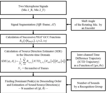
(20)where φ^S and θ^S are the estimated azimuth and elevation angles of a source, respectively. For multiple SSL, various peak detection strategies are applicable when multiple peaks in the SDE are present. However, since our research focused on a single SSL, we used the simplest global peak detection using equation (20). Figure 9 shows the proce‐ dure of the proposed SSL algorithm.
Figure 9. The proposed SSL algorithm based on SDE. Two measured
time-domain signals are divided into the given number of frames, Nf, and each
frame has Nfft samples. The shift angle corresponding to the middle sample in each frame is allocated to each frame. The framed signals are then used to calculate RxFxR(τ|θshift). Next, by using the constructed ICTD trajectory
database, the SDE can be obtained for every direction. Finally, by finding the dominant peak(s) in SDE in descending order, the source direction(s) can be estimated.
4. Simulation
In section 4, we evaluate the performance of the proposed SSL algorithm using synthesized signals. To do this, signal models of the fixed and rotating microphones were needed. These models are given in section 4.1 and the results of the simulation for a single source are described in section 4.2. The localization performance is evaluated with respect to the localization error, which is defined as the angle between the true and perceived direction vectors. In this simulation, the physical dimensions of the rotating microphone array are given in Table 1.
4.1 Signal Models of the Fixed and Rotating Microphones
As shown in Figure 3, the rotating microphone array is installed on a spherical head with a radius of rH. One of the two microphones is fixed at (−rH, 0, 0) on the surface of the spherical head (this microphone is hereafter called the “fixed microphone” for convenience). Then, the output signal of the fixed microphone in a continuous time domain, denoted as xF(t), can be modelled as below:
( )
xF( )
T*(
,)
F S S S
x t =h t s tj q (21)
where hSxF(t) is the spherical impulse response [25] from the source position to the fixed microphone position on the spherical head, s(t
|
φs, θs) is the source signal contents, and* indicates the convolution operator. As shown in equation (21), hSxF(t) is not a function of θshift because this microphone
does not move. However, the other microphone (i.e., the rotating microphone) is located on the rotating plate and moves in a circular motion on theYRZR plane (see Figures
2 and 3). Then, the measured signal of the rotating micro‐ phone should be strongly dependent on the shift angle. The signal model of the rotating microphone denoted as xR(t) can be defined as:
( )
R(
Shift) (
* ,)
T x R S S S x t =h tq s tj q (22) where hSxR(
t|
θshift
)
is the spherical impulse response fromthe source position to the rotating microphone position. In this case, hSxR is a function of θshift due to its circular motion.
The synthesized signal refers to the discrete-time domain signal. The generation of the synthesized signal of the fixed microphone, denoted as xF n, is carried out by simply discretizing xF(t), as shown below:
(
)
F F S
x né ù =ë û x n tD (23)
where ΔtS is the sampling time and xF n is the nth sample of the synthesized signal of the fixed microphone. On the other hand, the motion of the rotating microphone makes the generation of xRn more complicated. For example,
when we assume that the rotating microphone is shifted +θN° in a clockwise direction from the +ZR axis and fixed during the measurement, then the output signal xR(t) of the rotating microphone is:
(
shift)
R(
shift) (
* ,)
T x
R N S N S S
x tq =q =h tq =q s tj q (24)
By using this notation, M xR(⋅), which is the matrix of conditioned (continuous) output signals, can be modelled as equation (25) and is composed of Nf output signals with ΔθN degree resolution:
( )
(
)
(
)
(
)
(
)
shift shift shift 0 1 R R N R R f N x t x t Mx x t N q q q q q é = ù ê ú ê = D ú ê ú × = ê ú ê ú = - × D ê ú ë û M (25)where xR
(
t|θshift)
is equal to xR(
t|θshift+ 2π)
due to the circular motion of the rotating microphone, which means a cyclo-stationary process when a source content is station‐ ary [26]. We assume that the other dimensions do not vary. In this simulation, we set the sampling frequency (fS) and the number of frames (Nf) as 44.1 kHz and 360, respectively. Thus, ΔθN becomes 1°, and M xR ⋅ , which is the matrix ofconditioned discretized signals, can be modelled in equation (26):
(
)
(
)
(
)
(
)
shift shift shift 0 , 1 R S R S N R f N R S f N x n t x n t Mx N x n t N q q q q q q é D = ù ê ú ê D = D ú ê ú é D ù= ë û ê ú ê ú D = - × D ê ú ë û M (26)From equation (26), the synthetized signal of xRn along the shift angle axis can be represented as follows:
(
)
(
shift 1)
R R S N
x né ù =ë û x n tD q = n- × Dq (27) For instance, when the source is located in the direction of
(
φs, θs)
=(
0o, 0o)
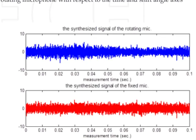
and its signal content is a Gaussian whitenoise signal, the resulting values included in Mxs ⋅ are presented in Figure 10. It is found that the amplitude of the synthesized signal is increasing as the shift angle of the rotating microphone gets close to 90° and is generally decreasing as the shift angle becomes close to 270°. This is a reasonable result: when the rotating microphone ap‐ proaches the source direction, the measured signal must be less attenuated by the spherical head. In this simulation model, the angular velocity of the rotating plate is 600 rpm. The synthesized output signal of the rotating microphone is collected along the signal detection line with wR of 600 rpm. In this case, the synthesized microphone outputs are presented in Figure 11.
4.2 Simulation Results
Various criteria to evaluate the SSL performance have been suggested by previous researchers [4, 6, 11-12, 15, 20]. One of the most commonly used criteria is based on the absolute error between true and perceived directions and it can be applied to the evaluation of azimuth or elevation angle estimations separately. However, for the evaluation of 3-D SSL performance, it would be more reasonable to incorpo‐ rate both azimuth and elevation together. If we express the perceived (or estimated) azimuth and levation angles as φ^S and θ^S respectively, then the true and perceived direction vectors (tdv→, pdv→) are defined with respect to the inter-aural polar coordinate:
(
)
$ $ $ $ $
(
sin ,sin , cos ,cos , sinsin)
S S S S S S S S S S tdv cos cos pdv cos cos j j q j q j j q j q = = uuur uuuur (28)
Figure 10. M xR ⋅ of conditioned and discretized output signals of the rotating microphone with respect to the time and shift angle axes
Figure 11. The synthesized output signals of the rotating and fixed
microphones are xR n (top) and xF n (bottom), respectively
Using these definitions, the localization error is defined as cos−1tdv→, pdv→. For example, when a Gaussian white noise
rotating period, GCC-PHAT functions corresponding to the circular motion of the rotating microphone were shown in Figure 12. Each GCC-PHAT function was calculated by using the segments of the synthesized signals of the two microphones. These segments have 1,024 (i.e., Nfft) samples
and there are 900 overlapping samples between adjacent frames. The meaningful region in the time domain is from - 1.4⋅10−3 seconds to + 1.4⋅10−3 seconds. It is found that the
peak location of the GCC-PHAT function moves up and down in the time domain, as expected (see section 2.2). In the situation where one fixed sound source is at (0o, 0o), the
peak position is the highest in the time domain when θshift
is equal to 90o and is the lowest when θshift is 270o. No other
significant features were found because additional noise signals were not included in the synthesized signals.
Figure 12. The GCC-PHAT functions when the source is located directly at
the front side (0o, 0o). As we expected, the up-and-down pattern of the peak
location is clearly visible. In this noise-free simulation of a single source, there are no distinguishing local peaks along the time axis.
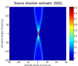
By using equation (19), SDE is obtained using the GCC-PHAT functions and the database of the approximated ICTD trajectories. Figure 13 shows the calculated SDE. The dominant peak is quite visible and bell-shaped side edges originating from the peak are spread out primarily along the elevation angle axis. This result is due to several factors. If the time resolution is infinitesimally small, the bell-shaped edges become invisible. However, the acquisition or processing system has its limitations, such as finite fS. As a result, adjacent ICTD trajectories may overlap each other. More specifically, the locations of the peaks of the GCC-PHAT functions are matched with more than one ICTD trajectory partially in the time domain. Thus, the side edges become visible. Also, we can expect that as the time interval increases, the overlapped region will expand and the SDE values corresponding to the side edges will increase. Secondly, even if SDE is calculated in the discrete-time
domain with a denser time resolution, the side edges should appear, because the signal bandwidth is limited. Thus, it can be expected that the calculated GCC-PHAT function is not equal to an ideal impulse. Besides, the effect of the rotational motion on the synthesized signals remains, although it is not remarkable. Therefore, the processing in the discrete-time domain and the motion of the rotating microphone cause the bell-shaped edges.
We examined the 3-D SSL performance of the proposed SSL algorithm for a Gaussian white noise source with respect to the localization error as mentioned above. The range of the source direction is as follows: its azimuth angle spans from -90° to +90° with 10° intervals and its elevation angle varies from 0° to +330° (-30°) with 30° intervals. The number of source directions is 228. It is assumed that the rotating microphone array system was located in a free field. Figure 14 shows the localization error distribution for all of the source directions. Generally, the performance gets better as the source is close to the left, opposite to the rotating microphone, due to the left and right asymmetry of the azimuth-dependent ICTD trajectory amplitude (see Figure 8). Also, it is reasonable that an elevation-dependent feature was not visible. The distribution of the mean errors along the azimuth angle was shown in Figure 15.
4.3 Computational load comparison
To be an efficient 3-D SSL method, the signal processing costs must be light. In this section, the computational load of the proposed localization method is compared with those of the delay-and-sum beamformer [27] and the steered response power (SRP) – PHAT method [28]. For example, SRP-PHAT requires the frequency-domain processing to do the phase transform (PHAT). Here, if the Figure 13. SDE for the source at the front side of the rotating array is shown.
It was found that the dominant peak is around the true direction of the source (0o, 0o). Additionally, the bell-shaped side edges originated from the
peak due to the regional overlap of adjacent ICTD trajectories. The shape of the peak is stretched in the direction of the elevation angle axis due to the short up-and-down motion of the rotating microphone, compared with the width of the array.
number of microphones is denoted as M, the computation of all the possible GCC-PHAT functions requires M(M-1)/2 phase transforms. For a discrete Fourier transform size of
Nfft, a single FFT takes 5Nfftlog2Nfft operations.
1. DFT of the all the microphones: M Χ (5Nfftlog2Nfft)
2. Spectral processing: 7NfftM(M-1)/2
3. Inverse DFT: M(M-1)/2 Χ (5Nfftlog2Nfft)
4. SRP-PHAT calculation for possible directions (NφNθ): M(M-1)/2 Χ NφNθ
position is the highest in the time domain when
equal to 90o and is the lowest when ߠ
ୱ୦୧୲other significant features were found because additional
noise signals were not included in the synthesized signals.
By using equation (19), SDE is obtainedusing
PHAT functions and the database of the
ICTD trajectories. Figure 13 shows the calculated SDE.
The dominant peak is quite visible and bell
edges originating from the peak are spread out
along the elevation angle axis. This result is due to
several factors.If the time resolution is infinitesim
small, the bell-shaped edges become invisible. However,
the acquisition or processing system has its limitations
such as finite f
S. As a result, adjacent ICTD trajectories
may overlap each other. More specifically, the locations
of the peaks of the GCC-PHAT functions are matched
with more than one ICTD trajectory partially in
domain. Thus, the side edges become visible. Also,
can expect that as the time interval
overlapped region will expand andthe
corresponding to the side edges will increase.
even if SDE is calculated in the discrete-time domain with
a denser time resolution, the side edges should
because the signal bandwidth is limited. Thus, it can
expected that the calculated GCC-PHAT function is not
equal to an ideal impulse. Besides,the effect of the
rotational motion on the synthesized signals remain
although itisnot remarkable. Therefore, the processing in
the discrete-time domain and the motion of the rotating
microphone cause the bell-shaped edges.
We examined the 3-D SSL performance of the
SSL algorithm for a Gaussian white noise source
respect to the localization error as mentioned above. T
range of the source direction isas follow
angle spans from -90
oto +90
owith 10
ointerval
Figure 13.SDE for the source at the front side of the rotating array is shown. It was found that the dominant peak is around the true direction of the source (0୭, 0୭
). Additionally, the bell shaped side edges originated from the peak due to the regional overlap of adjacent ICTD trajectories. The shape of the peak is stretched in the direction of the elevation angle axis due to the short up-and-down motion of the rotating microphone
position is the highest in the time domain when ߠ
ୱ୦୧୲is
ୱ୦୧୲is 270o. No
other significant features were found because additional
noise signals were not included in the synthesized signals.
using the
GCC-functions and the database of the approximated
shows the calculated SDE.
bell-shaped side
spread out primarily
This result is due to
If the time resolution is infinitesimally
shaped edges become invisible. However,
the acquisition or processing system has its limitations,
adjacent ICTD trajectories
. More specifically, the locations
PHAT functions are matched
with more than one ICTD trajectory partially in the time
domain. Thus, the side edges become visible. Also, we
can expect that as the time interval increases, the
the SDE values
will increase. Secondly,
time domain with
should appear,
the signal bandwidth is limited. Thus, it can be
function is not
the effect of the
rotational motion on the synthesized signals remains,
not remarkable. Therefore, the processing in
time domain and the motion of the rotating
D SSL performance of the proposed
SSL algorithm for a Gaussian white noise source with
o the localization error as mentioned above. The
follows:its azimuth
intervals and its
the front side of the rotating array is shown. It was found that the dominant peak is around . Additionally, the bell-shaped side edges originated from the peak due to the regional
ies. The shape of the peak is stretched in the direction of the elevation angle axis due to the the rotating microphone,
Figure 14.Localization errors for 228 directions are depicted. As we can see, the elevation-dependent feature was not found. However, it was quite visible that the SSL performance is strongly dependent on the azimuth angle of a source only.
elevation angle varies from 0
oto +330
intervals. The number of source directions is 228.
assumed that the rotating microphone array system was
located in a free field.Figure 14 shows
error distribution for all of the
Generally, the performance gets better as the source
close to the left, opposite to the rotating microphone
to the left and right asymmetry of the azimuth
ICTD trajectory amplitude (see Figure 8). Also, it is
reasonable that an elevation-dependent feature
visible. The distribution of the mean errors along the
azimuth angle was shown in Figure 1
4.3 Computational load comparison
To be an efficient 3-D SSL method, the signal processing
costs must be light. In this section, the computational
load of the proposed localization method is compared
Figure 15.The mean error along the azimuth angle of a source. The localization errors of the left-sided sources are almost the same, except for the leftmost source. The right
tend to be estimated with worse resolution compared
-90 -60 -30 0 30 0 1 2 3 4 5 6 7 8
azimuth angle of a source (degree)
M e a n a b s o lu te e rr o r (d e g re e )
Mean error distribution for sources on a sagittal plane
Localization errors for 228 directions are depicted. As dependent feature was not found. However, it was quite visible that the SSL performance is strongly dependent on the azimuth angle of a source only.
to +330
o(-30
o) with 30
osource directions is 228. It is
assumed that the rotating microphone array system was
shows the localization
of the source directions.
the performance gets better as the source is
rotating microphone, due
to the left and right asymmetry of the azimuth-dependent
igure 8). Also, it is
dependent feature was not
he mean errors along the
igure 15.
D SSL method, the signal processing
costs must be light. In this section, the computational
proposed localization method is compared
The mean error along the azimuth angle of a source. sided sources are almost the except for the leftmost source. The right-sided sources tend to be estimated with worse resolution compared with the
60 90
azimuth angle of a source (degree)
Mean error distribution for sources on a sagittal plane
Figure 15. The mean error along the azimuth angle of a source. The
localization errors of the left-sided sources are almost the same, except for the leftmost source. The right-sided sources tend to be estimated with worse resolution compared with the left-sided sources.
Figure 14. Localization errors for 228 directions are depicted. As we can see,
the elevation-dependent feature was not found. However, it was quite visible that the SSL performance is strongly dependent on the azimuth angle of a source only.
Thus, the total SRP-PHAT processing cost is M(M+1)/2 X
5Nfftlog2Nfft + M(M-1)/2 X (NφNθ + 7Nfft). In the same way, the cost of the proposed localization algorithm is (3M-1)/2 X
5Nfftlog2Nfft+ (M-1) X (NφNθ+ 7/2Nfft) and the cost of the delay-and-sum beamformer is MN X (NφNθ) where N is the frame length, 100. Therefore, the approximated costs are computed: (1) delay-and-sum beamformer, MN (NφNθ), (2) SRP-PHAT method, M2(N
φNθ+12Nfft), (3) the proposed method, M (NφNθ+9/2Nfft). It is noteworthy that if the Nfft is
smaller than NφNθ, the signal processing cost of the proposed localization method is N or M times less than the delay and sum beamformer and SRP-PHAT methods. It is reasonable that the proposed localization cue can be computed by M microphone pairs when using the (M+1)-channel microphone array. However, when using the SRP-PHAT method, the M(M-1)/2 microphone pairs are utilized for a single localization process. On the other hand, it is known that the SRP-PHAT method can be applied to the situation where the signal to noise ratio (SNR) is less than zero. However, in the proposed localization method, the TDE error will have an effect directly on the localization performance because the proposed cue is based on the measured ICTD trajectory. Thus, it can be reasonably expected that the proposed localization performance will be significantly more degraded than that of the SRP-PHAT method when SNR<0.
5. Experiment
We developed a rotating microphone array according to the proposed design (see Figure 2 and Table 1). It should be noted that the two microphone signals needed to be transmitted wirelessly for safety reasons. Thus, both a microphone and a transmitter needed to be placed inside the rotating block. An ultrasonic motor was chosen to make this block rotate inside the head. Details about the structure of the proposed array and the measurement process are provided in section 5.1. Section 5.2 shows the results of the two experiments for the feasibility test: one involving a Gaussian white noise source and the other involving a voice source.
Figure 16. A top view of the hemisphere showing the interior arrangement
of the rotating and fixed blocks, two ultrasonic motors, one encoder, and one motor driver. The rotating block on the right side contains the electronic boards for transmitting the microphone signal. The shift angle of the rotating microphone is measured by using the encoder.
5.1 Experimental Set-up
For our proposed rotating microphone array, we chose a wireless system (Q240, RFQ) consisting of a dual-channel receiver, two transmitters, and two microphones (QB686, RFQ). In order to put a transmitter unit and a microphone together in a rotating block, the electronic boards inside the transmitter unit had to be rearranged and installed in a cylindrical plastic block. Figure 16 shows the interior arrangement of the necessary blocks and other units inside the spherical head. There are two cylindrical blocks, two ultrasonic motors, one encoder, and one motor driver. The cylindrical block on the right side is called the “rotating block” and this block consists of the rearranged electronic boards used to transmit the microphone signal (#. 1) and the pin-type microphone located 3 cm from the centre of the cap. This block is connected to the ultrasonic motor (USR-E3T/24V, SHINSEI), which is driven by the motor driver (D6060E, SHINSEI). Additionally, the encoder is attached to the motor. Thus, the shift angle of the micro‐ phone is measured using the encoder signal. The other block on the left side is hereafter called the “fixed block” for convenience. The pin-type microphone (#. 2) is attached at the centre of the cap. The transmitter unit is outside the block. The left and right side views are also presented in Figure 17. The physical dimensions are the same as those in Table 1, except the rotating radius rR, which is 3 cm in the real array. Therefore, the ICTD trajectory database needed to be reconstructed.
with those of the delay-and-sum beamformer [27] and the steered response power (SRP) – PHAT method [28]. For example, SRP-PHAT requires the frequency-domain processing to do the phase transform (PHAT). Here, if the number of microphones is denoted as M, the computation of all the possible GCC-PHAT functions requires M(M-1)/2 phase transforms. For a discrete Fourier transform size of Nfft, a single FFT takes
5Nfftlog2Nfft operations.
1. DFT of the all the microphones: M Χ (5Nfftlog2Nfft)
2. Spectral processing: 7Nfft M(M-1)/2
3. Inverse DFT: M(M-1)/2 Χ (5Nfftlog2Nfft)
4. SRP-PHAT calculation for possible directions (NφNθ):
M(M-1)/2 Χ NφNθ
Thus, the total SRP-PHAT processing cost is M(M+1)/2 X 5Nfft log2 Nfft +M(M-1)/2 X (NφNθ + 7Nfft). In the same way,
the cost of the proposed localization algorithm is (3M-1)/2 X 5Nfft log2 Nfft + (M-1) X (NφNθ + 7/2Nfft) and the cost of
the delay-and-sum beamformer is MNX (NφNθ) where N
is the frame length, 100. Therefore, the approximated costs are computed: (1) delay-and-sum beamformer, MN (NφNθ), (2) SRP-PHAT method, M2 (NφNθ+12Nfft), (3) the
proposed method, M (NφNθ +9/2Nfft). It is noteworthy that
if the Nfftis smaller than NφNθ, the signal processing cost
of the proposed localization method is N or M times less than the delay and sum beamformer and SRP-PHAT methods. It is reasonable that the proposed localization cue can be computed by M microphone pairs when using the (M+1)-channel microphone array. However, when using the SRP-PHAT method, the M(M-1)/2 microphone pairs are utilized for a single localization process. On the other hand, it is known that the SRP-PHAT method can be applied to the situation where the signal to noise ratio (SNR) is less than zero. However, in the proposed localization method, the TDE error will have an effect directly on the localization performance because the proposed cue is based on the measured ICTD trajectory. Thus, it can be reasonably expected that the proposed localization performance will be significantly more degraded than that of the SRP-PHAT method when SNR<0.
5. Experiment
We developed a rotating microphone array according to the proposed design (see Figure 2 and Table 1). It should be noted that the two microphone signals needed to be transmitted wirelessly for safety reasons. Thus, both a microphone and a transmitter needed to be placed inside the rotating block. An ultrasonic motor was chosen to make this block rotate inside the head. Details about the structure of the proposed array and the measurement process are provided in section 5.1. Section 5.2 shows the results of the two experiments for the feasibility test: one involving a Gaussian white noise source and the other involving a voice source.
Figure 16. A top view of the hemisphere showing the interior arrangement of the rotating and fixed blocks, two ultrasonic motors, one encoder, and one motor driver. The rotating block on the right side contains the electronic boards for transmitting the microphone signal. The shift angle of the rotating microphone is measured by using the encoder
5.1 Experimental Set-up
For our proposed rotating microphone array, we chose a wireless system (Q240, RFQ) consisting of a dual-channel receiver, two transmitters, and two microphones (QB686, RFQ). In order to put a transmitter unit and a microphone together in a rotating block, the electronic boards inside the transmitter unit had to be rearranged and installed in a cylindrical plastic block. Figure 16 shows the interior arrangement of the necessary blocks and other units inside the spherical head. There are two cylindrical blocks, two ultrasonic motors, one encoder, and one motor driver. The cylindrical block on the right side is called the “rotating block” and this block consists of the rearranged electronic boards used to transmit the microphone signal (#. 1) and the pin-type microphone located 3 cm from the centre of the cap. This block is connected to the ultrasonic motor (USR-E3T/24V, SHINSEI), which is driven by the motor driver (D6060E, SHINSEI). Additionally, the encoder is attached to the motor. Thus, the shift angle of the microphone is measured using the encoder signal. The other block on the left side is hereafter called the “fixed block” for convenience. The pin-type microphone (#. 2) is attached at the centre of the cap. The transmitter unit is outside the block. The left and right side views are also presented in Figure 17. The physical dimensions are the same as those in Table 1, except the rotating radius ݎோ , which is 3 cm in
the real array. Therefore, the ICTD trajectory database needed to be reconstructed.
(a) (b)
Figure 17. The right-side view of the spherical head is shown in the left and the left-side view is presented in the right.
Figure 17. The right-side view of the spherical head is shown in the left and
the left-side view is presented in the right
5.2 Experimental Results
The experiments for the feasibility test were carried out in the room environment: the room size was 3.2 x 5.5 x 2.8 m3 (width x length x height) and the reverberation time was
0.26 seconds (t60). The input signal was produced through a full range speaker (TC9FSD13, VIFA) on the speaker jig. Figure 18 shows the rotating array system placed in the room. Two experiments were conducted in order to check the feasibility: one involving a Gaussian white noise signal and the other using a male voice as a source signal.
5.2.1 Gaussian white noise source
First, the experiment using a Gaussian noise source as an input signal to the speaker was conducted. In this experi‐
ment, the SSL performance for a source in the median plane was evaluated. Only the elevation angle of a source was varied from -30° to 210° with 10° intervals. The source content was Gaussian white noise signal with frequency contents from 1.5 kHz to 20 kHz generated by the random noise generator (SF-06, RION) and was produced longer than the one rotating period. The angular frequency was set to 54 rpm. For example, when the source is at (0o, 0o),
the measured microphone signals and the z-phase encoder signal are depicted in Figure 19. The total measurement time was 3 seconds and the signal duration was set to 2 seconds. By using the encoder signal in the z-phase, we collected the samples within a single rotating period and allocated Nfft samples to each frame. For 25 directions in the
median plane, the mean localization error was 1.75° and the standard deviation was 1.65°. Therefore, the experimental result showed that our proposed SSL algorithm is applica‐ ble to the SSL of a Gaussian noise source.
Figure 19. The output signals of two microphones and the encoder signal
(z-phase) when the source is at (0o, 0o)
Figure 18. The spherical head equipped with the rotating microphone array
5.2.2 Male voice source
The previous experiment employed a Gaussian white noise signal as a source. In this experiment, a male voice was used as the sound source, without using a speaker jig. The male’s position was fixed during the measurement so that his mouth was at (45°, 0°) while speaking. The angular frequency of the rotating block was reduced to 21 rpm in order to involve the silent region. The output signals of the two microphones and the encoder signal are depicted in Figure 20. It is known that voice signals are not stationary with time. Also, the spectral modification is strongly dependent on the relative position of the sensor and the source. If the microphones are not attached on an object such as a sphere, but located in the free field, the spectral contents in the measured microphone signals will be the same. Figure 21 shows the GCC-PHAT functions along the shift angle of the rotating microphone. In the region where sufficient signal contents were collected, the GCC functions were obtained quite reasonably because the peak location seemed to change in a sinusoidal form. The empty black-coloured circles show the estimated ICTDs.
Figure 20. The output signals of two microphones and the encoder signal
(z-phase) in the time domain when the voice source is at (45o, 0o). As shown,
the voice signal is non-stationary.
Figure 21. The GCC-PHAT functions along the shift angle of the rotating
microphone. In the region with sufficient signal contents, the functions were obtained easily. This can be interpreted to mean that the peak location of each function is shifting up and down as the rotating microphone moves in a circular motion. The more smoothed peaks result from the comparatively narrow frequency band of the measured voice signals.
Figure 22 shows the SDE for all possible directions with 2° resolution on both the azimuth and elevation directions. Consequently, the dominant peak in the SDE was found. As we examined earlier, bell-shaped side edges originate from the peak. Negative values were found at some regions. This result seems reasonable because a GCC function can have a negative value, which indicates that considerable contents in the measured signals are out-of-phase with each other. The final step to find the location of the (positive) peak in the SDE was carried out to estimate the direction of a source as equation (20).
Figure 22. The source direction estimator when a source was at (45o, 0o).
The estimated source direction was (39o, −1o) even though the silent
region was included. 6. Discussion
The concept of the proposed localization cue, which is a (source) direction- and (microphone) position-dependent ICTD trajectory, can be applied to the circular microphone array as well. In general, if a microphone array is composed of (M+1) sensors, all the information from every possible microphone pair is under consideration, in order to practically improve the SSL resolution. If the M-channel circular microphone array is located on the right side of the sphere and the one additional microphone is fixed on the other side, the (microphone which is the element of the M-channel circular array) position-dependent ICTD trajectory can be reproduced exactly the same as the proposed ICTD trajectory. Thus, the proposed localization cue-based 3-D SSL can be also applicable to the circular microphone array. However, the more microphones that are used for SSL, the more costly it is to produce the microphone array, espe‐ cially due to the price of the Analog-to-Digital converters (ADC), which is proportional to the number of channels. However, sequential sampling and signal processing could be an alternative to reduce the production cost.
On the other hand, the source position was supposed to be outside the rotating microphone array. However, noises