Impact Angle Control Guidance Synthesis for Evasive Maneuver against Intercept Missile

(1)

Received: May 12,2017 Revised: September 7, 2017 Accepted: September 11, 2017

719

http://ijass.org pISSN: 2093-274x eISSN: 2093-2480

Paper

Int’l J. of Aeronautical & Space Sci. 18(4), 719–728 (2017) DOI: http://dx.doi.org/10.5139/IJASS.2017.18.4.719

Impact Angle Control Guidance Synthesis for Evasive Maneuver against

Intercept Missile

Y. H. Yogaswara*

Korea Advanced Institute of Science and Technology, Daejeon 34141, Republic of Korea Department of Research and Development of Indonesian Air Force, Bandung 40174, Indonesia

Seong-Min Hong and Min-Jea Tahk*

Korea Advanced Institute of Science and Technology, Daejeon 34141, Republic of Korea

Hyo-Sang Shin****

Cranfield University, Bedford MK43 0AL, United Kingdom

Abstract

This paper proposes a synthesis of new guidance law to generate an evasive maneuver against enemy’s missile interception while considering its impact angle, acceleration, and field-of-view constraints. The first component of the synthesis is a new function of repulsive Artificial Potential Field to generate the evasive maneuver as a real-time dynamic obstacle avoidance. The terminal impact angle and terminal acceleration constraints compliance are based on Time-to-Go Polynomial Guidance as the second component. The last component is the Logarithmic Barrier Function to satisfy the field-of-view limitation constraint by compensating the excessive total acceleration command. These three components are synthesized into a new guidance law, which involves three design parameter gains. Parameter study and numerical simulations are delivered to demonstrate the performance of the proposed repulsive function and guidance law. Finally, the guidance law simulations effectively achieve the zero terminal miss distance, while satisfying an evasive maneuver against intercept missile, considering impact angle, acceleration, and field-of-view limitation constraints simultaneously.

Key words: Missile guidance, Evasive maneuver, Impact angle control, Artificial potential field

1. Introduction

Since an Integrated Air Defense Systems (IADS) [1] have been sophistically developed, a countermeasure action to counteract the IADS becomes a significant consideration in a missile design. Surface attack missiles, which are launched from air or surface platforms to attack designated surface targets also need advanced solutions to respond the threats of IADS. Guidance system design for surface attack missile in this high threat environment is challenging since the attacking missile must be delivered to its target, while maximizing the survivability from the IADS. A proper guidance laws to

generate an evasive maneuver against intercept missiles are rarely published in open literature. On the contrary, the evasive maneuver of manned aircraft against intercept missile has been studied extensively. Those evasive strategies are based on continuously changing maneuver direction such as barrel roll and the Vertical-S maneuver [2, p. 120] or weaving maneuver [2, Ch. 27]. The strategies are not adequate to be implemented into homing missiles or unmanned aerial vehicles (UAVs) due to several reasons, i.e.: the movement can be easily predicted, the maneuver might exceed seeker’s field-of-view (FOV) limitation, and the missile fails to satisfy zero terminal miss distance.

This is an Open Access article distributed under the terms of the Creative Com-mons Attribution Non-Commercial License (http://creativecomCom-mons.org/licenses/by- (http://creativecommons.org/licenses/by-nc/3.0/) which permits unrestricted non-commercial use, distribution, and reproduc-tion in any medium, provided the original work is properly cited.

* Ph. D Student, Research Officer ** Ph. D Student

*** Professor, Corresponding author: [email protected] **** Associate Professor

(2)

DOI: http://dx.doi.org/10.5139/IJASS.2017.18.4.719

₇₂₀

Int’l J. of Aeronautical & Space Sci. 18(4), 719–728 (2017)

An optimal evasive maneuver for subsonic Anti-Ship Missiles (ASM) has been studied against Close-in Weapon System (CIWS) [3]. The CIWS is a common short-range IADS for naval ships that are usually equipped with cannon as the defensive weapon. Since the ASM moves with constant acceleration at any moment, the CIWS is able to aim at the predicted intercept position. In [3], the authors have defined a time-varying weighted sum of the inverse of the aiming errors as a cost function which to be minimized. Inspired by the study above, a direct optimization technique using Co-Evolutionary Augmented Lagrangian Method (CEALM) was applied in [4], which the capturability analysis is proven using Lyapunov-like approach. Both studies in [3] and [4] generate a type of barrel roll evasive maneuver, however, a large barrel roll maneuver could increase the miss distance at the terminal time.

As studied in [5], the typical CIWS’s cannon system has limitations due to single-threat-engagement capability and fire at a predicted intercept point of the threat’s trajectory. This limitation motivates a new guidance law by using salvo attack where multiple missiles are launched and guided to arrive at a stationary target at the same desired time. The guidance law adopting this idea has been firstly proposed by Jeon et al. in [6] and called as Impact Time Control Guidance (ITCG). To control the impact time, the ITCG suggests an additional loop in a closed form solution based on the linear formulation of traditional proportional navigation guidance (PNG) law. The ITCG has been also proposed in [7] by introducing a virtual leader approach. Sliding mode control (SMC) method for ITCG has been adopted in [8]. A Lyapunov-based law is the latest method proposed in [9] for ITCG and simultaneous arrival.

Even though the ITCG has been broadly studied, the concept of salvo attack for simultaneous impact time by exploiting the limitation of CIWS is less effective. In fact, if we may be allowed for a little exaggeration, it is not applicable anymore. This knowledge is exposed since CIWS or IADS introduces intercept missiles to enhance the previous cannon system. The intercept missile has advanced capability of multi-target engagement, longer intercept range, and proximity warhead detonation for a higher probability of kill. Regarding those new developments, this paper proposes a new guidance law, which maximizes survivability of an attack missile with respect to the threat of advanced CIWS or IADS. In order to neutralize the threat of intercept missile of enemy’s IADS, our attack missile must have an evasive maneuver capability to counteract the interception. In addition, the attack missile must satisfy an impact angle constraint and zero terminal acceleration for maximizing warhead detonation effect on the target. FOV

limitation of the attack missile is also considered to ensure the seeker locks on the target.

Due to its elegant concept and simple computation, the evasive maneuver of the attack missile in this paper is based on the concept of Artificial Potential Field (APF). The APF was introduced by Krogh [10] and Khatib [11] for mobile robots by defining functions of goal attractive potentials and obstacle repulsive potentials. Inherent problems of APF were systematically identified by Koren and Borenstein in [12] due to a trap situations caused by local minima, no passage between close space obstacle, and oscillation. In addition, Goal Non-reachable with Obstacle Nearby (GNRON) problem was also recognized and solved by Ge and Cui in [13]. Modifications of APF for moving obstacles have been also proposed in [14]–[16]. Nevertheless, those modifications cannot be implemented to the missile problem since the modified potential functions require a deceleration variable to reduce velocity when facing the obstacle. Eventually, inspired by Chen et al. in [17], this paper proposes a new repulsive function that effective for the missile problem and overcomes the GNRON problem at the same time. The primary limitation of APF on trap situation due to local minima will not be an issue in this evasive maneuver scenario since the problem is one-on-one engagement with relatively free dead-end trajectory, e.g. U-shaped obstacle.

Regarding the concept of APF, instead of the conventional attractive potential function, this paper implements an impact angle control guidance (IACG) method as the attractive goal. The IACG attacks the weak spot of a target to increase warhead detonation effect and maximize its probability of kill towards the target. A generalized formulation of energy minimization had been proposed in [18] to achieve IACG. A PNG-based was proposed in [19] for capturing all possible terminal impact angle. Lyapunov-based pursuit guidance was introduced in [20] to reduce the angle between the velocity and the distance vector. A combination of differential game and sliding mode control were also proposed in [21]. The Time-to-go Polynomial Guidance (TPG) as proposed by Lee et al. in [22] which treat the guidance command as a function of time-to-go is the most suitable to be adopted in this paper. In addition to the impact angle constraint, the TPG also satisfies the zero terminal acceleration to minimize the terminal angle-of-attack (AOA) for effective impact angle, and zero terminal lateral velocity to minimize zero effort miss.

In order to improve the practicality on the physical concern of proposed guidance law, the limitation on actuator’s acceleration command is considered in this paper. Moreover, the seeker look angle is also limited to be inside the FOV in order to ensure the missile seeker not losing its target.

(3)

721

Y. H. Yogaswara Impact Angle Control Guidance Synthesis for Evasive Maneuver against Intercept Missile

http://ijass.org

Switching logic was implemented in [23] by switching the guidance law from ITCG of [6] to the second law of constant look angle guidance command, when the seeker look angle exceeds the FOV limit. A rule of the cosine of a weighted leading angle in the biased term was used in [24] to ensure the ITCG was satisfied without violating the FOV constraint during an engagement. Switching logic to constant seeker look angle was also investigated in [25] for optimal IACG of a missile with a strap-down seeker. Without applying the switching logic, SMC was used in [26] to satisfy IACG by implementing a control Integral Barrier Lyapunov Function (iBLF) to design the reaching law. The implementation of iBLF inspires this paper to apply a simpler internal penalty function known as Logarithmic Barrier Function (LBF) to limit the look angle.

This paper is organized as follows. Section 2 presents the new proposed repulsive potential functions of APF with its properties. In Section 3, the equations of motion, APF, TPG, LBF and all corresponding problem formulation are synthesized to generate a single acceleration command of proposed guidance law. Guidance characteristics, analysis, and solutions are presented in Section 4 by numerical simulation at a particular missile engagement scenario. The simulations successfully demonstrate the effectiveness of the potential function and guidance law. Finally, concluding remarks and future works are given in Section 5.

2. Proposed Repulsive Potential Function

The repulsive potential function that is implemented on mobile robots, robot manipulators, and UAVs are broadly based on the Khatib [11] or Ge and Cui [13]. However, those repulsive potential functions are not suitable to be used in missile engagement problem due to its potential characteristics. The main properties of those functions is a steep slope of repulsive potential, which the potential values ascent sharply approaching the obstacle position. This property is acceptable for mobile robots since it has the capability of deceleration when approaching the obstacle, stop the movement, and reroute its path. Conversely, the missiles engagement scenario does not recognize those capabilities.

The repulsive potential function for missile engagement scenario needs a gradual ascent of potential approaching the obstacle to anticipate the intercept in advance. The gradual and gentle ascent of repulsive potential has been introduced for UAV path planning by Chen et al. in [17]. Unfortunately, this function does not consider the GNRON problem, which drives a failure to achieve the goal position. The failure is

generated by shifting out the global minimum from the goal position when the goal is within the influence distance of the obstacle.

A new repulsive potential function of APF is constructed and proposed to generate a gradual ascent of potential approaching the obstacle and solve the GNRON problem at the same time. Assuming a generic problem of a point masses vehicle, goal, and obstacle, which the vehicle moves in a two-dimensional (2-D) space. The vehicle position in the workspace is denoted by

5

problem formulation are synthesized to generate a single acceleration command of proposed guidance law. Guidance characteristics, analysis, and solutions are presented in Section 4 by numerical simulation at a particular missile engagement scenario. The simulations successfully demonstrate the effectiveness of the potential function and guidance law. Finally, concluding remarks and future works are given in Section 5.

2. Proposed Repulsive Potential Function

The repulsive potential function for missile engagement scenario needs a gradual ascent of potential approaching the obstacle to anticipate the intercept in advance. The gradual and gentle ascent of repulsive potential has been introduced for UAV path planning by Chen et al. in [17]. Unfortunately, this function does not consider the GNRON problem, which drives a failure to achieve the goal position. The failure is generated by shifting out the global minimum from the goal position when the goal is within the influence distance of the obstacle.

A new repulsive potential function of APF is constructed and proposed to generate a gradual ascent of potential approaching the obstacle and solve the GNRON problem at the same time. Assuming a generic problem of a point masses vehicle, goal, and obstacle, which the vehicle moves in a two-dimensional (2-D)

space. The vehicle position in the workspace is denoted by q=

[

x y_A _A

]

T. The repulsive potential

U q

_rep

( )

at each vehicle position is defined by considering the relative distance of goal position into Chen’s equation as follow goal, if ( ) 0, if obst d obst o rep obst o e d d d U d d ζ e −  ≤  =  >  q (1) . The repulsive potential 5

[

x y_A _A

]

U q

rep

( )

at each vehicle position is defined by considering the relative distance of goal position into Chen’s equation as follow goal, if ( ) 0, if obst d obst o rep obst o e d d d U = e −ζ _d ≤_d >  q (1)

at each vehicle position is defined by considering the relative distance of goal position into Chen’s equation as follow

5

[

x y_A _A

]

U q

_rep

( )

at each vehicle position is defined by considering the relative distance of goal position into Chen’s equation as follow goal, if ( ) 0, if obst d obst o rep obst o e d d d U d d ζ e −  ≤  =  >  q (1) , (1) 6 goal goal obst obst d d = − = − q q q q (2)

where d_obst,

d

goal, d0,

e

, and ζ are the minimal distance between the vehicle and the obstacle, the

distance between the vehicle and the goal, the distance of influence of the obstacle, and both are positive design parameter gains, respectively. This proposed function ensures the repulsive potential approaches zero as the vehicle approaches the goal and finally the goal position will be the global minimum of total potential.

The effectiveness of the proposed repulsive potential function is demonstrated in a case on

one-dimensional (1-D) space as shown in Fig. 1. The vehicle q=

[

xA 0

]

Tis moving along x-axis toward the

goal

[

4 0

]

T

goal=

q while avoiding the obstacle qobst=

[

0 0

]

T. Assuming the distance of influence of the

obstacle d = , the GNRON problem of the predecessor function as mentioned by Chen et al. in [17] is ₀ 6

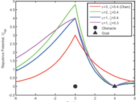
demonstrated in the first plot series. Since the goal position near the obstacle, the generated repulsive potential is large enough to create the non-reachable goal. This problem takes place since the goal position is affected by the obstacle and drive non-zero potential at the goal. Moreover, the potentials are evenly distributed to the right and the left side of the obstacle neglecting the goal. In the same case assumption, the new proposed function shows significant improvement to handle the GNRON problem. The plot of three different combinations of scaling gains maintains the minimum of the potential at the goal position and the maximum of the potential at the obstacle position. Furthermore, the scaling gains show the freedom to control the properties of repulsive potential. The higher value of e, the higher peak value of the potential. The higher value of ζ, the steeper ascent of potential approaching the obstacle.

-6 -4 -2 0 2 4 6 -0.5 0 0.5 1 1.5 2 2.5 3 3.5 4 4.5 5 Position, x R epul si ve P ot ent ial , Ure p e=3, ζ=0.4 (Chen) e=2, ζ=0.4 e=1, ζ=0.4 e=1, ζ=0.3 Obstacle Goal

Fig. 1. Repulsive potential function in a 1-D space

The corresponding repulsive force is given by the negative gradient of the repulsive potential. According

to Eq.(1), when the vehicle is not at the goal, i.e.,

q q

≠

goal, the repulsive force is given by

,

(2)

where dobst, dgoal, d0, ε, and ζ are the minimal distance

between the vehicle and the obstacle, the distance between the vehicle and the goal, the distance of influence of the obstacle, and both are positive design parameter gains, respectively. This proposed function ensures the repulsive potential approaches zero as the vehicle approaches the goal and finally the goal position will be the global minimum of total potential.

The effectiveness of the proposed repulsive potential function is demonstrated in a case on one-dimensional (1-D) space as shown in Fig. 1. The vehicle

6 goal goal obst obst d d = − = − q q q q (2)

where d_obst,

d

goal, d0,

e

[

xA 0

]

goal qgoal=

[

4 0

]

T while avoiding the obstacle qobst =

[

0 0

]

q q

≠

is moving along x-axis toward the goal

where d_obst,

d

goal, d0,

e

[

xA 0

]

goal

[

4 0

]

T

goal=

q while avoiding the obstacle q_obst=

[

0 0

]

q q

≠

_goal, the repulsive force is given by

while avoiding the obstacle

where d_obst,

d

goal, d0,

e

[

x_A 0

]

goal qgoal=

[

4 0

]

T while avoiding the obstacle

[

0 0

]

T obst=

q . Assuming the distance of influence of the

q q

≠

. Assuming the distance

of influence of the obstacle d0=6, the GNRON problem of the

predecessor function as mentioned by Chen et al. in [17] is demonstrated in the first plot series. Since the goal position near the obstacle, the generated repulsive potential is large enough to create the non-reachable goal. This problem takes place since the goal position is affected by the obstacle and

where d_obst,

d

_goal, d0,

e

one-dimensional (1-D) space as shown in Fig. 1. The vehicle

_q

=

[

x

_A

0 ]

goal qgoal=

[

4 0

]

q

obst

=

[

0 0

]

obstacle d =₀ 6, the GNRON problem of the predecessor function as mentioned by Chen et al. in [17] is

demonstrated in the first plot series. Since the goal position near the obstacle, the generated repulsive potential is large enough to create the non-reachable goal. This problem takes place since the goal position is affected by the obstacle and drive non-zero potential at the goal. Moreover, the potentials are evenly distributed to the right and the left side of the obstacle neglecting the goal. In the same case assumption, the new proposed function shows significant improvement to handle the GNRON problem. The plot of three different combinations of scaling gains maintains the minimum of the potential at the goal position and the maximum of the potential at the obstacle position. Furthermore, the scaling gains show the freedom to

control the properties of repulsive potential. The higher value ofe, the higher peak value of the potential. The

higher value ofζ, the steeper ascent of potential approaching the obstacle.

q q

≠

(4)

DOI: http://dx.doi.org/10.5139/IJASS.2017.18.4.719

₇₂₂

Int’l J. of Aeronautical & Space Sci. 18(4), 719–728 (2017)

drive non-zero potential at the goal. Moreover, the potentials are evenly distributed to the right and the left side of the obstacle neglecting the goal. In the same case assumption, the new proposed function shows significant improvement to handle the GNRON problem. The plot of three different combinations of scaling gains maintains the minimum of the potential at the goal position and the maximum of the potential at the obstacle position. Furthermore, the scaling gains show the freedom to control the properties of repulsive

potential. The higher value of ε, the higher peak value of

the potential. The higher value of ζ, the steeper ascent of

potential approaching the obstacle.

The corresponding repulsive force is given by the negative gradient of the repulsive potential. According to Eq.(1), when the vehicle is not at the goal, i.e.,

where d_obst,

d

goal, d0,

e

[

x_A 0

]

goal qgoal=

[

4 0

]

[

0 0

]

T obst=

q . Assuming the distance of influence of the

q q

≠

goal, the repulsive force is given by the repulsive force

is given by 7

(

)

( ) ( ) , if ( ) 0, if rep rep

repObst obst repGoal goal obst o rep obst o F U F F d d F _d _d = −∇ + ≤  =  _>  q q n n q (3) obst d repObst goal

F

₌

_eζ

d e

−ζ (4) obst d repGoal

F

₌

_e

e

−ζ (5)

where _n_obst= ∇d_obst and ngoal= −∇dgoal are unit vectors pointing from the obstacle to the vehicle and from

the vehicle to the goal, respectively. Those unit vectors play an important role since the nobst repulses the

vehicle away from the obstacle and the

n

goal attracts the vehicle towards the goal.

To elaborate the properties of the force field, the case on Fig. 1 is developed into 2-D space, which the

scaling gains are defined as

e

=20 and ζ =0.3. The repulsive potential field and repulsive force field of

the vehicle at every position in a 2-D space are depicted in Fig. 2. The repulsive potential field keeps the goal as the global minima and the potential peak at the obstacle. The repulsive potential force represents the potential as a positive divergent vector field outward the obstacle and a negative divergent vector field inward the goal. Intuitively, the vehicle that affected by this vector field will be repulsed by the obstacle and attracted to the goal.

-6 -4 -2 0 2 4 6 -10 0 10 0 10 20 30 40 50 60 70 80 90 Y X R epul si ve P ot ent ial , Ure p Obstacle Goal -4 -3 -2 -1 0 1 2 3 4 5 -4 -3 -2 -1 0 1 2 3 4 X Y Repulsive Force Obstacle Goal

Fig. 2. Repulsive potential field (left) and repulsive force field (right) in a 2-D space

Regarding the implementation of the new repulsive function into missile evasive maneuver, some nomenclatures are adjusted. The vehicle of interest, the obstacle and the goal are defined as the attack missile, the intercept missile, and the target, respectively.

3. Guidance Synthesis

Consider a two-dimensional homing guidance scenario as shown in the left illustration of Fig. 3. The , (3) 7

(

)

( ) ( ) , if ( ) 0, if rep rep

F

₌

_eζ

d e

−ζ ₍₄₎ obst d repGoal

F

₌

_e

e

−ζ (5)

where _n_obst= ∇d_obst and n_goal= −∇d_goal are unit vectors pointing from the obstacle to the vehicle and from

the vehicle to the goal, respectively. Those unit vectors play an important role since the n_obst repulses the

n

e

Consider a two-dimensional homing guidance scenario as shown in the left illustration of Fig. 3. The

, (4) 7

(

)

( ) ( ) , if ( ) 0, if rep rep

F

₌

_eζ

d e

F

₌

_e

e

−ζ (5)

the vehicle to the goal, respectively. Those unit vectors play an important role since the _n_obst repulses the

n

e

, (5) where 7

(

)

( ) ( ) , if ( ) 0, if rep rep

F

₌

_eζ

d e

F

₌

_e

e

−ζ (5)

n

e

Consider a two-dimensional homing guidance scenario as shown in the left illustration of Fig. 3. The and 7

(

)

( ) ( ) , if ( ) 0, if rep rep

F

₌

_eζ

d e

F

₌

_e

e

−ζ (5)

where _n_obst= ∇d_obst and _n_goal= −∇d_goal are unit vectors pointing from the obstacle to the vehicle and from

n

e

Consider a two-dimensional homing guidance scenario as shown in the left illustration of Fig. 3. The are unit vectors

pointing from the obstacle to the vehicle and from the vehicle to the goal, respectively. Those unit vectors play an

important role since the

7

(

)

( ) ( ) , if ( ) 0, if rep rep

repObst obst repGoal goal obst o rep obst o F U F F d d F d d = −∇ + ≤  =  _>  q q n n q (3) obst d repObst goal

F

₌

_eζ

d e

F

₌

_e

e

−ζ ₍₅₎

the vehicle to the goal, respectively. Those unit vectors play an important role since the n_obst repulses the

n

e

Consider a two-dimensional homing guidance scenario as shown in the left illustration of Fig. 3. The repulses the vehicle away from

the obstacle and the

7

(

)

( ) ( ) , if ( ) 0, if rep rep

F

₌

_eζ

d e

F

₌

_e

e

−ζ (5)

n

e

Consider a two-dimensional homing guidance scenario as shown in the left illustration of Fig. 3. The attracts the vehicle towards the

goal.

To elaborate the properties of the force field, the case on Fig. 1 is developed into 2-D space, which the scaling gains

are defined as ε=20 and ζ=0.3. The repulsive potential field

and repulsive force field of the vehicle at every position in a 2-D space are depicted in Fig. 2. The repulsive potential field keeps the goal as the global minima and the potential peak at the obstacle. The repulsive potential force represents the potential as a positive divergent vector field outward the obstacle and a negative divergent vector field inward the goal. Intuitively, the vehicle that affected by this vector field will be repulsed by the obstacle and attracted to the goal.

3. Guidance Synthesis

Consider a two-dimensional homing guidance scenario as shown in the left illustration of Fig. 3. The friendly attack

missile has a constant velocity VA heading to enemy’s

stationary target while avoiding enemy’s intercept missile,

1

1. Affiliation’s postcode (우편번호) of 1st_author:

Department of Research and Development of Indonesian Air Force, Bandung 40174, Indonesia

2. Affiliation’s postcode (우편번호) of 4th_author:

Cranfield University, Bedford, MK43 0AL, United Kingdom

3. Change right figure of Fig. 3 (simplified vector):

Fig. 3. Guidance geometry (left) and guidance synthesis of acceleration command vector (right)

7

(

)

( ) ( ) , if ( ) _0, _if rep rep

F

₌

_eζ

d e

F

₌

_e

e

−ζ (5)

where n_obst = ∇d_obst and _n_goal = −∇d_goal are unit vectors pointing from the obstacle to the vehicle and from

n

e =

20

and ζ =0.3. The repulsive potential field and repulsive force field of

Impact Angle Control Guidance Synthesis for Evasive Maneuver against Intercept Missile

719

Paper