Husimi functions at gradient index cavities
designed by conformal transformation optics
I
NBOK
IM,
1J
INHANGC
HO,
1Y
USHINK
IM,
2B
UMKIM
IN,
2J
UNG-W
ANR
YU,
3S
UNGHWANR
IM,
4ANDM
UHANC
HOI1,*1School of Electronics Engineering, Kyungpook National University, Daegu 41566, South Korea 2Department of Mechanical Engineering, Korea Advanced Institute of Science and Technology, Daejeon 34141, South Korea
3Center for Theoretical Physics of Complex Systems, Institute for Basic Science (IBS), Daejeon 34051, South Korea
4School of Electrical and Computer Science, Gwangju Institute of Science and Technology, Gwangju 500-712, South Korea
Abstract: Dielectric cavity systems, which have been studied extensively so far, have uniform refractive indices of their cavities, and Husimi functions, the most widely used phase space representation of optical modes formed in the cavities, accordingly were derived only for these homogeneous index cavities. For the case of the recently proposed gradient index dielectric cavities called as transformation cavities designed by optical conformal mapping, we show that the phase space structure of resonant modes can be revealed through the conventional Husimi functions by constructing a reciprocal virtual space. As examples, the Husimi plots were obtained for an anisotropic whispering gallery mode (WGM) and a short-lived mode supported in a limaçon-shaped transformation cavity. The phase space description of the corresponding modes in the reciprocal virtual space is compatible with the far-field directionality of the resonant modes in the physical space.
© 2018 Optical Society of America under the terms of the OSA Open Access Publishing Agreement
OCIS codes: (140.3945) Microcavities; (230.5750) Resonators; (000.3860) Mathematical methods in physics; (260.2710) Inhomogeneous optical media.
References and links
1. E. J. Post, Formal Structure of Electromagnetics (Wiley, 1962).
2. J. Plebanski, “Electromagnetic waves in gravitational fields,” Phys. Rev. 118(5), 1396–1408 (1960). 3. I. V. Lindell, Methods for Electromagnetic Field Analysis (Oxford University, 1992).
4. J. B. Pendry, D. Schurig, and D. R. Smith, “Controlling electromagnetic fields,” Science 312(5781), 1780–1782 (2006).
5. O. Ozgun and M. Kuzuoglu, “Form Invariance of Maxwell’s Equations: The Pathway to Novel Metamaterial Specifications for Electromagnetic Reshaping,” IEEE Antennas Propag. Mag. 52(3), 51–65 (2010). 6. Y. Liu and X. Zhang, “Recent advances in transformation optics,” Nanoscale 4(17), 5277–5292 (2012). 7. Y. Kim, S. H. Lee, J. W. Ryu, I. Kim, J. H. Han, H. S. Tae, M. Choi, and B. Min, “Designing whispering gallery
modes via transformation optics,” Nat. Photonics 10(10), 647–652 (2016).
8. U. Leonhardt, “Optical Conformal Mapping,” Science 312(5781), 1777–1780 (2006). 9. L. Xu and H. Chen, “Conformal transformation optics,” Nat. Photonics 9(1), 15–23 (2015).
10. H. Cao and J. Wiersig, “Dielectric microcavities: Model systems for wave chaos and non-Hermitian physics,” Rev. Mod. Phys. 87(1), 61–111 (2015).
11. T. Harayama and S. Shinohara, “Two-dimensional microcavity lasers,” Laser Photonics Rev. 5(2), 247–271 (2011).
12. K. Husimi, “Some formal properties of the density matrix,” Proc. Phys.-Math. Soc. Jpn. 22, 264–314 (1940). 13. B. Crespi, G. Perez, and S.-J. Chang, “Quantum Poincaré sections for two-dimensional billiards,” Phys. Rev. E
Stat. Phys. Plasmas Fluids Relat. Interdiscip. Topics 47(2), 986–991 (1993). 14. H.-J. Stöckmann, Quantum Chaos (Cambridge University, 1999).
15. M. Hentschel, H. Schomerus, and R. Schubert, “Husimi functions at dielectric interfaces: Inside-outside duality for optical systems and beyond,” Europhys. Lett. 62(5), 636–642 (2003).
16. W. C. Chew, Waves and Fields in Inhomogeneous Media (Wiley-IEEE, 1999).
17. A. Bäcker, S. Fürstberger, and R. Schubert, “Poincare Husimi representation of eigenstates in quantum billiards,” Phys. Rev. E Stat. Nonlin. Soft Matter Phys. 70(3), 036204 (2004).
#315230 https://doi.org/10.1364/OE.26.006851 Journal © 2018 Received 8 Dec 2017; revised 25 Jan 2018; accepted 26 Jan 2018; published 7 Mar 2018
18. D. Liu, L. H. Gabrielli, M. Lipson, and S. G. Johnson, “Transformation inverse design,” Opt. Express 21(12), 14223–14243 (2013).
19. T. Needham, Visual Complex Analysis (Clarendon, 2002).
20. M. Robnik, “Classical dynamics of a family of billiards with analytic boundaries,” J. Phys. A 16(17), 3971–3986 (1983).
21. In preparation (to be published elsewhere).
1. Introduction
Maxwell's equations, the governing equations for electromagnetic fields in space-time including media, have fundamental symmetries under various transformations such as well-known Lorentz transformation and gauge transformation. Maxwell's equations are also form-invariant under general coordinate transformations [1–3]. Exploiting the form invariance of Maxwell's equations for general coordinate transformations, Pendry et al. theoretically presented transformation optics (TO) [4] which is a general methodology for designing electromagnetic materials including optical invisibility cloaks, and various photonic devices which manipulate the path of light waves [5, 6]. Particularly, very recently, applying the TO to the design of optical dielectric resonators, Kim et al. reported 2-dimensional (2D) gradient index dielectric cavities called transformation cavities by using conformal TO [7–9]. Surprisingly, in their transformation cavities, directional whispering gallery modes (WGMs) with very high quality factors (Q-factor) are possible, providing a great potential for cutting-edge optical device design.
Conventional 2D optical dielectric cavities with uniform refractive indices have been regarded as an open system version of closed quantum billiard systems and also as a potential candidate of low-threshold micro-lasers, so there have been vast and intensive works on these platform systems over the last twenty years [10, 11]. In order to analyze the characteristics of optical modes supported in 2D dielectric cavities, it is often more useful to represent the optical modes in phase space than merely depict the mode intensity patterns in real physical space. One of the popular phase space representations of a wave function is Husimi function, which can be regarded as a quasi-probability distribution in phase space. It is defined by the overlap of the wave function with a coherent state of a minimum uncertainty wave packet [12]. The so-called Poincaré Husimi functions on the billiards boundary have been widely used when studying quantum-classical correspondence in quantum billiards [13, 14]. For the case of optical 2D dielectric cavities, Hentschel et al. have derived four different Husimi functions in a reduced phase space, i.e., on the Poincaré surface of section (PSOS) at the dielectric interfaces by using a stationary phase approximation [15].
However, since the Husimi functions of Hentschel et al. are valid exclusively for homogeneous dielectric interfaces, it is inappropriate to apply their Husimi functions directly to the transformation cavities to see the phase space structure of optical modes formed there. In this paper, we show that the Husimi functions can still be useful for optical modes supported in transformation cavities with inhomogeneous refractive indices. To this end, we construct a virtual space which we call a reciprocal virtual (RV) space, through the inverse of the conformal mapping, then both polarized resonant modes supported in the transformation cavity of the physical space and the corresponding virtual modes in the unit disk cavity of the RV space turn out to be identical. Besides, the refractive index of the unit disk cavity in the RV space is uniform. Based on these facts, one can obtain a phase space description of the internal waves in a transformation cavity through the conventional Poincaré Husimi functions calculated in the RV space.
This paper is organized as follows. In section 2, starting from a uniform index unit disk cavity in a fictitious space called as an original virtual space we describe the gradient index transformation cavity model in physical real space. In section 3, RV space is introduced to apply conventional Husimi functions for the internal waves in a uniform index cavity. As an illustration of our method, Husimi functions for a directional high-Q WGM and a directional
low-Q mode in a limaçon-shaped transformation cavity are calculated and analyzed in section 4. In the last section comes our conclusion.
2. Gradient index cavities designed by optical conformal mapping
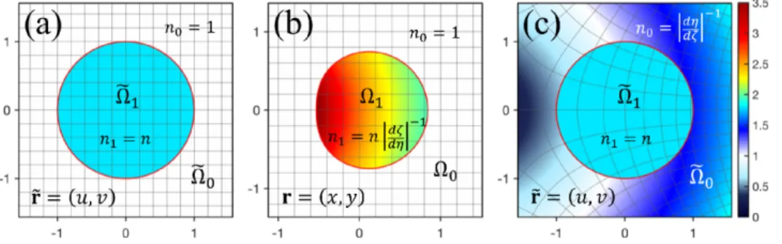
We start with a homogeneous dielectric cavity of an infinite cylinder with a unit disk cross section in an original virtual (OV) space with Cartesian coordinates ( , , )u v w , taking w-axis along the axis of the cylinder as shown in Fig. 1(a). In the OV space, the uniform refractive index of the cavity is n and the refractive index of the exterior region is 1 as the refractive index of vacuum or practically that of air. In the physical space with Cartesian coordinates ( , , )x y z , a realizable 2D gradient index cavity model (hereafter called as ‘transformation cavities’) can be built by applying a conformal coordinate transformation only to the inside region (Ω ) of the unit disk cavity in the OV space and assigning the uniform refractive index 1
of n0 =1 for the outside region (Ω0) of the transformed cylindrical cavity ( z w= ) with a deformed cross section as shown schematically in Fig. 1(b). For these transformation cavities with deformed shapes, it was demonstrated that directional WGMs called ‘conformal WGMs’ (cWGMs) can be formed [7]. The conformal coordinate transformation from the OV space to the physical space is given by an analytic function ζ = f( )η =x u v( , )+i y u v( , ) of a complex variable η= +u iv, that satisfies the Cauchy–Riemann equations,
,
x y y x
u v u v
∂ =∂ ∂ = −∂
∂ ∂ ∂ ∂ . (1)
Conformal mappings preserve angles locally; both angles and the shapes of infinitesimally small figures are preserved, but not necessarily their size or curvature. Also the handedness of coordinate system is unchanged.
Fig. 1. Schematic illustration of a transformation cavity and its pertaining two virtual spaces: (a) the unit disk cavity in an original virtual (OV) space, (b) a limaçon-shaped transformation cavity in the physical space, (c) the corresponding unit disk cavity in a reciprocal virtual (RV) space. (Refractive index profiles are expressed by common color scale.)
Due to the translation symmetry along the z-axis of the aforementioned cylindrical geometry, Maxwell’s equations simplify to a 2D scalar wave equation for the two polarization of light with respect to the z-axis [10]. Resonant modes in a transformation cavity with a deformed boundary are found by solving the following 2D scalar wave equation,
2( ) 2 ( ) 0 n k Δ ψ + = r r , (2) where 2 2 x y
Δ≡ ∂ + ∂ , position vector, r=( , ) ( cos , sin )x y = r θ r θ and the refractive index n r( ) is given by
1 1 0 , Ω (interior) ( ) 1 , Ω (exterior) d d n n ζ η − ∈ = ∈ r r r , (3)
with the radiation boundary condition,
( ) ~ ( , ) for i k r e h k r r ψ r θ → ∞, (4) where h( , )θ k is the far-field angular distribution of the radiation emission. The radiation boundary condition leads to solutions exponentially decaying in time with discrete complex eigenvalues k with Im[ ] 0k < . Complex angular frequency is ω =ck, where c is the speed of light in vacuum given by 1 ε μ0 0 . The lifetime τ of these so-called ‘resonant modes’ or
‘resonances’ is given by the imaginary part of the angular frequency as τ= −1 2 Im[ ]ω ; the quality factor of each resonance is defined by Q 2= π τ T = −Re[ ] 2 Im[ ]ω ω , where the oscillation period of light wave is T=2π Re[ ]ω . The complex wave function ψ( )r
represents Ez and Hz components with regard to the transverse magnetic (TM) and the transverse electric (TE) polarizations, respectively, i.e., the TM polarized time-harmonic electric field is given by ( , ) ( , z Re[ ( )) ˆ i t] zˆ
z
t =E t = ψ e−ω
E r r r and the TE polarized H-field is
given by ( , ) ( , z Re[ ( )) ˆ i t] zˆ z
t =H t = ψ e−ω
H r r r . The boundary conditions at the cavity–air interface are of a mixed type given by [10, 16]
1 0, 1 0 for TM modes ψ ψ= ∂⊥ψ = ∂⊥ψ , (5a) 1 1 0 2 0 1 , for TE modes n ψ ψ ψ ⊥ ψ ⊥ ∂ = = ∂ , (5b)
where ψj are wave functions on the cavity boundary from the interior region ( j=1) and the exterior region ( j=0) and ∂⊥ψj are their normal derivatives, respectively; ∂ ≡⊥ p r( )⋅∇|r
and ( )p r is the outward normal unit vector on the cavity boundary curve Γ at point r and
1
n is the gradually-varying refractive index along the boundary, i.e., n1=n dζ ηd −1
evaluated at the boundary.
3. Poincaré Husimi function at transformation cavities
The Husimi function, a quasiprobability distribution in phase space is originally defined as the overlap of the wave function with a coherent state that represents a minimal-uncertainty wave packet. Crespi et al. derived so-called a Poincaré Husimi function at the boundary of 2D
closed quantum billiard systems by projecting the conventional Husimi function from full 4-dimensional phase space onto a 2D reduced phase space, namely on the PSOS at the system boundary [13]. It has been widely used in the 2D billiard systems in the context of quantum chaos, especially in order to study the semiclassical regime [14, 17]. For the case of dielectric systems with piecewise constant refractive indices, Hentschel, et al. have derived four different Poincaré Husimi functions, corresponding to incident and emerging waves on inside and outside of the interface by using a semiclassical (saddle point) approximation with a Green’s function technique [15]. Among them, the Husimi functions for the internal waves have been useful when exploring ray-wave correspondence in optical dielectric cavities.
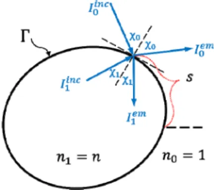
Fig. 2. Incident and emerging rays at a dielectric interface with uniform refractive indices.
Their expression for circular cavity can be readily extended to cavities with deformed boundaries as below. Four different Husimi functions which represent the intensities of the incident and emerging waves from arc length s along the cavity boundary Γ in the directions χj ( j=1; interior region, j=0; exterior region), respectively are (see Fig. 2)
2 ( )
0
( , sin ) ( 1) ( , sin ( ) ( , sin )
2 ) j inc em j j j j j j j j j k i H s h s h s k χ χ χ π ′ = − + − (6)
with weighting factors j= njcosχj and the functions h , j h′j given by
Γ , sin ( ; , sin ) ( ) ( ) j j j j h s χ =
ds′ψ s′ ξ s s′ χ , (7a) Γ ( ( , sin ) ) ( ; , sin ) j j j j h s′ χ =
ds′∂⊥ψ s′ ξ s s′ χ , (7b) which are the overlaps of the wave function ψ and its normal derivative ∂⊥ψ , taken on the respective sidej
of the cavity boundary, with the minimum-uncertainty wave packet2 4
1 ( 2 )
( ; , sin ) exp sin ( 2 )
2 j j j l s s l s s π ik s l ξ χ σ χ π σπ ∈ ′ − − + ′ = − ′+
, (8) which is periodic in s′ and centered around ( , sins χj). The uniform refractive index of interior region is n1=n and the refractive index of exterior region is n0=1; the kj are the wave number in each region. The width of the wave packet in the s-direction along with the uncertainty in sinχj can be controlled with the parameter σ = 2 k1.The boundary Husimi function of each region is valid when the refractive index is constant in each region. Therefore, in the case of the transformation cavities the Eq. (6) can be used for the exterior region where the refractive index is 1, but the formula cannot be directly applied to the interior region. However, fortunately, if we construct a virtual space through inverse conformal transformation, a transformation cavity is mapped back to the original unit disk cavity with the same uniform refractive index, so the boundary Husimi function for the resonant modes in the interior region can be calculated there by the above formula. In other words, it becomes possible to look at the phase space structure that shows the emission direction of the resonant modes and the location on the boundary where the major emission leaks out.
So, we introduce the reciprocal virtual (RV) space with Cartesian coordinates ( , , )u v w , which is obtained from the physical space by the inverse conformal mapping, η= f−1( )ζ , as
shown in Fig. 1(c). It is noted that the inverse conformal mapping is not a one-to-one mapping and therefore the RV space corresponding to the OV space should be selected. Functions, differential operators, and relevant symbols in the RV space will be expressed with tildes. Under the inverse conformal mapping, the scalar wave Eq. (2) is transformed to
2( ) 2 ( ) 0 n k Δ ψ + = r r , (9) where 2 2 u v
Δ ≡ ∂ + ∂ , position vector r=( , )u v , and refractive index n r( ) is given by
1 1 0 , (interior) ( ) , (exterior) d d n n η ζ − ∈Ω = ∈Ω r r r . (10)
Notice that the intracavity refractive index in the RV space is the same as that of the OV space but the exterior index varies spatially as shown in Fig. 1(c). Incidentally, if we take the RV space as an OV space, the transformation cavity in the physical space can be obtained from the RV space without artificial setting of n0=1 for the outside region.
In the RV space, the Husimi functions for the incident and the emerging waves in the unit disk cavity with uniform index n can be written as below.
2 ( ) 1 1 1 1 1 1 1 1 1 1 , sin , sin ( ) ( , si ( ) ( n ) 2 ) inc em k n H s h s i h s k χ χ χ π ′ = − + (11)
with weighting factor 1= ncosχ1 and the functions h1, h1′ given by
1( , sin 1) 1( ) ( ; , sin 1) h s χ ds ψ s ξ s s χ Γ ′ ′ ′ =
, (12a) 1( , sin 1) 1( ) ( ; ,sin 1) h s′ χ =
Γds′∂⊥ψ s′ ξ s s′ χ , (12b) which are the overlaps of the wave function ψ and its normal derivative ∂ ⊥ψ , taken on the inside ( j=1) of the unit disk cavity at arc length s along the boundary ′ Γ in the RV space, with the minimum-uncertainty wave packet2
1 4 1 1
1
( )
( 2 )
( ; , sin ) exp sin 2
2 l s s l s s π ik s l ξ χ χ π σ σπ ∈ ′ − − + ′ = − ′+
, (13) which is periodic in s and centered around ′ ( , sis nχ1). The parameter σ = 2 k1 controls the uncertainty in s and sinχ . For a resonant mode, 1 k1=nRe[ ]k where k is a complex wave number of the resonant mode.In order to calculate the Husimi function in the RV space, it is necessary to obtain ψ, ψ
⊥
∂ on the boundary of the unit disk cavity. To obtain these from the ψ , ∂⊥ψ along the boundary of a transformation cavity in physical space, we need to know the transformation rules between them. According to TO [4, 18], 3-dimensional transformation rules for electromagnetic fields and gradient operators between the physical space and the RV space can be expressed as follows,
1 1 1 (Λ−)T , (Λ−)T , (Λ−)T = = = E E H H ∇ ∇ . (14) where T, T x y z u v w = (∂ ∂ ∂ ) = (∂ ∂ ∂ )
∇ ∇ and the Jacobian matrix Λ and its inverse Λ−1 are
given by 1 0 0 0 , 0 0 0 1 0 0 1 x u x v u x u y y u y v v x v y Λ Λ− ∂ ∂ ∂ ∂ ∂ ∂ ∂ ∂ ∂ ∂ ∂ ∂ ∂ ∂ ∂ ∂ = = (15) because z w= , ∂ ∂ = ∂ ∂ =x w y w 0, and ∂ ∂ = ∂ ∂ =z u z v 0. Due to the Cauchy–Riemann equations, the scale factor of conformal mapping ζ = f( )η is given by det (Λ−1) which
equals dζ ηd −2 .
First of all, for TM and TE polarizations, wave functions in the physical space and their counterpart functions in the RV space are identical as can be shown by using the above field transformation rules; 0 0 0 0 0 0 0 0 1 u x v x u y v y ψ ψ ∂ ∂ ∂ ∂ ∂ ∂ ∂ ∂ = . (16)
So, ψ( , )x y =ψ( , )u v with x i y+ = f u iv( + ) between the physical space and the RV space. Secondly, from the complex analysis [19], the transformation rule between unit normal vectors px+i py and pu+i pv at the cavity boundaries in the respective spaces can be written as 1 ( ) x y u v d d d d p +i p = p +i p ζη ηζ − . (17)
Using the Cauchy–Riemann equations, Eq. (17) can be rewritten in 3-D Cartesian vector notation with ( 0)T x y p p = p and ( 0)T u v p p =
p as p=Λp detΛ . Thus, normal derivative transforms as 1 1 ( det ) T T d dζη Λ Λ Λ − − ⊥ ⊥ ∂ ≡ ⋅ =p ∇ p⋅ ∇ = ∂ . (18)
Therefore, through the relations ψ( )s =ψ ( )s and ∂⊥ψ( )s = dζ ηd −1∂ ⊥ψ( )s , one can obtain
the ψ, ∂ ⊥ψ on the boundary of the unit disk cavity in the RV space from the ψ , ∂⊥ψ on the boundary of a transformation cavity and calculate the Husimi functions (Eq. (11)) for the internal waves in the RV space.
4. Examples: a limaçon-shaped transformation cavity
As examples, we calculate the Husimi function for incident waves in the unit disk cavity in the RV space for a high-Q resonance (cWGM) and a low-Q resonance in a limaçon-shaped transformation cavity. The conformal mapping which transforms the unit circle to the limaçon [7, 20], is given by
2
( )
where η= +u iv and ζ = +x i y are complex variables that denote positions in the respective complex planes, is a deformation parameter, and β is a positive scaling factor. We use
0.23 =
, β =0.685, and n=1.8, the refractive index of unit disk cavity in the OV space. Wave functions of resonant modes formed in the transformation cavity can be calculated by a boundary element method (BEM) exploiting the RV space [7, 21] or finite element method (FEM) based electromagnetic field solvers e.g., COMSOL Multiphysics.
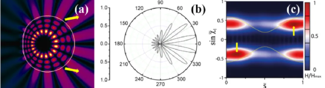
Fig. 3. A high-Q TM resonance (cWGM) in a limaçon-shaped transformation cavity (k=12.2333−i0.0022) (a) the mode intensity distribution; two yellow arrows denote the directions of tunneling emissions at s=0 in Fig. 3(c), (b) the far field pattern, (c) the intracavity Husimi plot for incident waves in the RV space; two yellow solid curves are critical lines of total internal reflection and the ± signs in sinχ denote the counterclockwise (CCW) 1
and clockwise (CW) circulations of light waves, respectively. (s is normalized with 2π, the total arc length of the unit disk cavity.)
Using the BEM, we obtained a high-Q TM mode which is identified as a cWGM with a complex wave number k=12.2333−i0.0022. The Q-factor of the resonance is 2776.23. The mode intensity distribution, the far field pattern and the intracavity Husimi function for incident waves are depicted in Fig. 3 (s is normalized with 2π, the total arc length of the unit disk cavity). As can be seen in Fig. 3(a), the cWGM is well confined by total internal reflection of light around the rim of the limaçon-shaped transformation cavity and this feature is reflected in the Husimi plot as the two band-type intensities located in the regions
1
1 ( )
sinχ > d dη ζ s−r n where the r.h.s. of the inequality represents the critical lines of total
internal reflection depicted by two yellow solid curves in Fig. 3(c) (the ± signs in sinχ1
denote counterclockwise (CCW) and the clockwise (CW) circulations of light waves, respectively). The bi-directional far field emission shown in Fig. 3(b) can be explained by the Husimi plot in the RV space in Fig. 3(c); the closest position between the intensity bands and critical lines in s is s=0 or 1 which corresponds to the position ( , ) (0.842 ,0)x y = 55 on the boundary of the limaçon-shaped transformation cavity where maximum evanescent leakage or tunneling emissions come out in tangential directions i.e., parallel to the y-axis [7].
Also, we obtained a low-Q TM mode with k=12.5960−i0.1302 whose intensity pattern is depicted in Fig. 4(a). The Q-factor of the resonance is 48.37. The far field emission shown in Fig. 4(b) is refractive emission as can be seen clearly from the Husimi plot in Fig. 4(c) where the intensity peaks of CW and CCW waves are located below the critical lines, i.e., in the regions sinχ1 d dη ζ s1( ) n
−
< r
. To analyze this refractive emission approximately, we resort to Snell’s law, n1sinχ1=sinχ0 in the physical space. Because of conformality of the transformation, one can take sinχ1=sinχ1~ 0.385,− the peak position of lower intensity in the Husimi plot. The peak position in s coordinate is s=0.1256 which can be converted into s=0.1732, normalized value with the whole boundary length of the limaçon. The
intracavity refractive index at this position is n1=1.9314. So, the refraction angle,
0 48.04
χ = − ° is obtained from 0
sinχ ~ 0.7436.− In polar coordinate, angular coordinate of the main emission point on the boundary of the limaçon-shaped transformation cavity is 0.929 (rad) or 53.226° and the outward normal direction at the point is 58.93 .° Thus, we can conclude that the main refractive emission comes out at the boundary point of angular coordinate 53.226° in the direction 10.89 .° By the mirror symmetry with respect to the x-axis, the peak of upper intensity in the Husimi plot corresponds to the refractive emission at the boundary point of angular coordinate −53.226° in the direction −10.89°. Thus the far field pattern in Fig. 4(b) can be understood as the interference of the two dominant (out of phase) refractive emission.
Fig. 4. A low-Q TM resonance in a limaçon-shaped transformation cavity (k=12.5960−i0.1302) (a) the mode intensity distribution; two yellow arrows designate dominant refractive emissions at the corresponding peak positions s=0.1256 and
0.8744
s= in the Husimi plot of Fig. 4(c), (b) the far field pattern, (c) the intracavity Husimi plot for incident waves in the RV space; two yellow solid curves are critical lines of total internal reflection same as in Fig. 3(c) and two yellow arrows point the intensity peaks of CW and CCW waves ( s is normalized with 2π, the total arc length of the unit disk cavity.)
5. Conclusion
A method to find a widely used phase space representation i.e., the Husimi representation for the internal waves on the boundary of a transformation cavity was presented by constructing a virtual space with a uniform dielectric cavity via inverse conformal transformation. As a verification of the method, Husimi plots for a high-Q and a low-Q resonance were obtained in the virtual space and their emission characteristics could be revealed from the plots. The phase space description of the corresponding modes in the virtual space agrees well with the far-field directionality of the resonant modes of a transformation cavity in the physical space. We expect that our method will be useful in studying waves in transformation cavities. Funding
National Research Foundation of Korea (NRF) grant funded by the Korea government (MSIP) (No. 2017R1A2B4012045 and No. 2017R1A4A1015565); Center for Advanced Meta-Materials (CAMM) funded by Korea Government (MSIP) as Global Frontier Project (CAMM 2014M3A6B3063709); Institute for Basic Science in Korea (IBS-R024-D1).
Acknowledgments