Control of Inverted Pendulum Using Continuous Time Deadbeat Control

(1)

ICCAS2005 June 2-5, KINTEX, Gyeonggi-Do, Korea

1. INTRODUCTION

A deadbeat controller is well-known in digital control system but can ‘t be applied to continuous time system because of it’s asymptotic property. So special method, for example delay elements method, must be used in continuous time system which is studied well by Japan researchers[1]-[3].

Additionally digital deadbeat control can be used. Firstly easily designed digital type controller is applied to the lower order smoothing element which is method suggested by Murata[4]-[8]. So the smoothed control output has the same effect of continuous time deadbeat controller. This smoothing element is the output of the controller and also is an input of the plant. If this smoothing element is regarded as one of plant elements, then plant including smoothing element become an argumented system. So digital deadbeat compensator must be firstly designed so that this argumented system attains digital deadbeat property. By S/W calculations two compensators are determined from this digital deadbeat controller. In references, researchers called this controller as CDBC(Continuous time DeadBeat Controller).

In this paper, we study on the CDBC implemented digitally which is suggested by Murata[4]-[8]. Especially, ZOH(Zero-order Hold) is applied to the digital deadbeat control and then resulted output is applied to the 2nd order smoothing element. As target plant rotary type 4th order inverted pendulum is used. Two unstable poles are relocated to LHP by using pole placement algorithms. Simulation is done using Matlab. DC servo motor is used to drive the pendulum.

2. CDBC THEORY

2.1 Continuous Time Parameters

Among various methods to obtain continuous time deadbeat control input, standard type second order delay elements are used for smoothing [4]-[7]. 2 2 2 2 ) ( n n n l w s w s w s G + + = ζ (1) Here

ζ

is a damping factor and

ω

nis a natural frequency.

2.2 Problem Statements

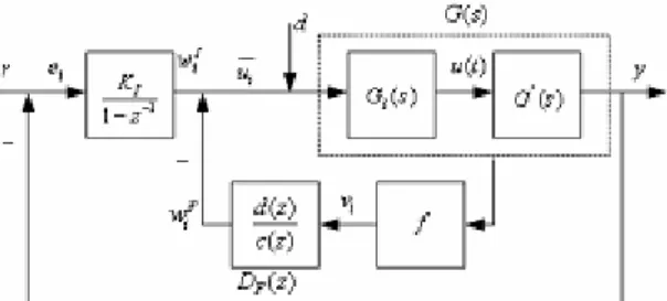
To make continuous time deadbeat controller in the control system block of Fig. 1, DF(z) is introdueced in local state

feedback loop and D_I(z) is also introuduced in the forward path as a form of serial feedforward form. This makes type 1 digital deadbeat control system[4]-[8].

Digital control input

u

iis obtained in an optimal sense.

And with symmetric weighing matrix, 2nd order performance index to be minimized is as follows[4]-[8].

₍ ₎ 2 1 k T kRu u Qe T e P= + (2)

Here

u

_kis control input which minimizes the index.

Fig. 1. Continuous time deadbeat control system

According to the rules,

u

i is firstly calculated to meet the

argumented system’s desired response and then for this control input, feedback compensator in the local feedback and integral compensator in the forward path are cacluated accordingly.

3. DEDIGN OF CDBC

3.1 Derivation of CDBC

Assume digital deadbeat controller’s control stage just before fininte time settling is

N

, and plant order, n and smoothing element’s order, 2 and additional degree of freedom as k

Geneally for small

N

, large control input is obtained and user must

Control of Inverted Pendulum Using Continuous Time Deadbeat Control

Ho-Jin Lee, Seung-Youal Kim,Jung-Kook Lee, Jin-Yong Kim, Seung-Hwan Lee, Keum-Won Lee and Jun-Mo Lee

Division of Electronic and Information Communication Engineering , Kwandong University, Gangnung, Korea (Tel : +82-33-670-3396; E-mail: [email protected])

Abstract: Due to the asymptotic property, deadbeat control can hardly be applied to the continuous time system control. But some delay element method can deal such a problem. Besides delay element method, well-known digital deadbeat control can be used by the aid of some smoothing elements. In this paper, 2nd order smoothing element is used for the smoothing of the digital deadbeat controller. And this element is argumented to the plant, and so control problem is to control the argumented system digitally. We simulated this control system using Matlab language and finally apply this algorithm to the rotary inverted pendulum system. Keywords: Continuous-time Deadbeat Controller, Smoothing elements, Inverted Pendulum, Pole Placement.

(2)

consider the size of

N

.

So N=n+2+k

(

k≥0

)

, and by the control input

(

i

=

0 ~

N

−

1 )

u

i after

N

stage

y

i

=

1 .

0 (

i

≥

N

)

,

(

≥

1 )

=

+

u

α

u

N a N . In this case, input-output relations are

_J

_u

k k r y = (3)

[

_u

]

u

k= 0 1... N ⎥ ⎥ ⎥ ⎥ ⎥ ⎦ ⎤ ⎢ ⎢ ⎢ ⎢ ⎢ ⎣ ⎡ ⋅ ⋅ ⋅ ⋅ ⋅ ⋅ ⋅ ⋅ = + + + + + + + + + + + + + − h g g g g g h g g g g g g g g g g J n n n n n N n N n n N N n n N N k 2 3 4 2 5 2 1 2 1 2 3 4 1 1 2 3 1 ... ... ... ... 0 ... ... ← k →← (n+3) → (4) Here

_g

iis impulse response sequence and is obtained from uinit

step response as

_g

_h

i i

i= − −1. In Eq. (4) impulse response sequences

of inverted pendulum’s argumented system are included. And output

(

i+N~N+n+2

)

y

i

must be

y

_r

=

[

111 ...

1 ]

T (5) In minimum-time continuous deadbeat control case

(

k

=

0 )

, Eq. (4) and Eq. (5) are reduced to

u

₀

=

J

₀−1

y

_r

=

[

u

₀

,

u

₁

,...

u

_n₊₂

]

(6) If

k

≥

1

, from Eq. (4)

rankJ

k

≠ n

+

3 and

u

kis not

determined uniquely. So from Eq. (5) by using constraints of

0 =

−

_k _k

r

J

u

y

and

Lagrange undetermined coefficients method, control input is calculated as follows[8].

[

]

[

]

[

]

[

]

T N r T k T k k T k r T k u u u i Qi G M J J M J J Qi G M u ... 1 0 1 1 1 1 = − − = − − − − (7)

[

]

[ ]

T r T

i

QG

G

R

M

=

+

,

=

1 ...

1

, 3.2 Design of CDBC

In Fig. 1 unit step function is used as reference input. Forward and feedback compensators are set as follows.

) 2 ( 2 1 1 ) 1 ( 1 1 1 ) 1 ( 1 1 1 0

...

)

(

...

1 )

(

...

)

(

)

(

)

(

)

(

+ − + − − − − − − − − −

+

=

+

=

+

=

n n N N N N F

z

d

z

f

z

f

z

c

z

c

z

c

z

d

z

d

z

d

z

c

z

d

z

D

(8)

If

i

=

0

, initial value of integral forward compensator is 0 and

u

I 0 0=

ω

. So gain of integrator

u

K

_I ≡ 0

. If unit step input is applied as a reference input, closed-loop response is as follows

(

)

0

(

)

(

)

/(

1

)

− − =

u

z

b

z

y

(9)

Here one of denominator terms is regarded as follows

{

1 (

)

(

)

(

)

}

(

)

1 )

1 (

−

z

−1

+

a

z

+

d

z

f

z

+

u

₀

b

z

=

(10)

So closed-loop transfer response is simplified as Eq. (9)[8]. In Eq. (10) polynomial

a,

b

have zero constant terms and have a degree of

N

. To obtain these polynomials in case of

n

= N

2 ,

=

5

, coefficient of powers from (-1) to (-9) are orders as follows.

0 0 0 0 ) ( 0 ) ( ) ( 0 ) ( ) ( 0 ) ( ) ( 0 ) ( ) ( 0 ) 1 ( 4 4 3 4 4 3 4 4 2 4 3 3 4 2 3 4 4 3 1 4 2 3 3 2 4 1 2 4 3 3 4 2 5 5 0 1 3 2 2 3 1 4 0 1 4 2 3 3 2 4 1 4 5 4 0 1 2 2 1 3 0 1 3 2 2 3 1 4 0 3 4 4 0 1 2 2 1 3 0 1 3 2 1 3 0 2 3 2 0 1 0 1 1 2 0 1 2 1 0 1 0 1 = − = − − = − − − + = − − − − + + + − = + − − − − + + + + − = + − − − + + + + − = + − − − + + + − = + − + + − = + + − f d f d f d f d f d f d f d f d f d f d f d f d f d f d f d f d a b u f d f d f d f d f d f d f d f d a a b u f d f d f d f d f d f d f d a a b u f d f d f d f d f d f d a a b u f d f d f d a a b u f d a (11) From Eq. (11), , , 0 4 3 2

f

=

f

because

_d

_i

≠

0

. So pulse

sequence transfer function

_D

_F

( )

z is as follows

( )

)} 1 ( 1 1 1 2 1 1 1 ) 1 ) 1 ( 1 1 1 1 ) 1 ( 1 1 1 ) ( ... ) ( { 1 1 /( ) ... ) 1 /( ... ( − − − − − − − − − − − − − − − − − − + + − + + = − + + + − + + + = − N N F N F F F N N N N N F n n F F z F w w z w w w v z z v v z v z w z w w z Z Z N Z N

D

(12) Coefficients in Eq. (12) are determined as follows by comparing the corresponding coefficients in

ω

_iI, _y

_u

0 , [8] 0 1 1 0 0 0 1 , , ) 1 ( u f b u y u y i u w i j j i i i j j F i ⎟⎟− = = ⎠ ⎞ ⎜ ⎜ ⎝ ⎛ − +

_∑

= = (13)

4. MODELLING OF ROTARY INVERTED

PENDULUM

The configuration of Rotary Inverted Pendulum is shown in Fig. 2. Measurements of angles

θ

,

φ

are done by using encoders with resolution 1024(pulse),2000(pulse) respectively.

(3)

Fig. 2 Rotary type pendulum

Pendulum’s model is described as follows by simplifying energy relations[11].

θ

cos 2 l g m PE_total = _b (14) ] ) ( [ 2 1

_φ

2

_φ

.

_θ

.

_θ

.2 ex b b t total J mlr J J KE = + + + (15)

Here

_J

_t

=

_J

_Arm

+

_m

_b

_r

2

+

_J

_m

+

_J

_ez . Above simplifed equations are combined to derive the next two equations by using Lagrangian Equations [9]. ) sin cos ( 2 1 .. . ..

θ

φ

−

=

j mlr T _t _b

(16) .. .. ) ( sin 2 1 cos 2 1 0

=

m_blr

φ

θ

−

m_bg

θ

+

J_b

+

J_ex

θ

(17)

Approximate values such as

θ

=

0 ,

sin

θ

=

θ

,

θ

&

=

0

are used with Eq. (16) and Eq. (17) and then after pole relocation to derive the following transfer function

1600 720 196 24 053 . 8 ) ( 2 3 4 2

+

−

=

s s s s s G s (18)

5. SIMULATION

5.1 Simulation(CDBC)

An inverted pendulum is naturally unstable system and is relocated using pole placement alogorithm in which new poles are

)

10 ,

464 .

3

2 (

−

±

j

−

. Overall augumented system

prepositioned by smoothing element is as follows

)

1600

720

196

24 )(

2 (

)

053 .

8 (

)

(

2 3 4 2 2 2 2

+

−

=

s

w

s

w

s

w

s

G

n n n

ζ

(19) Fig. 3 shows digital deadbeat control input which is applied to

augmented system with initial value [0 0 0 0.1 0 0 ]‘ in case of shortest settling stage 6 and digital control input is

]

9 .

1

9 .

8 ,

0 .

94

9 .

234 ,

8 .

82

8 .

403

5 .

403 [

]

[

₀ ₁ ₂ ₃ ₄ ₅ ₆ 0

−

=

T

u

(20)

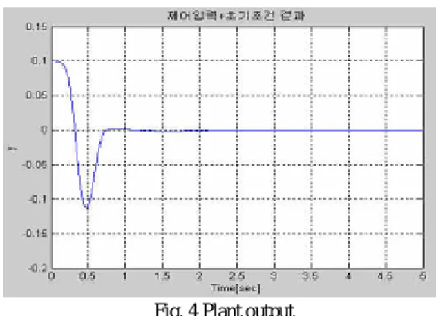
Fig. 4 shows resulting system output. Sampling time is set to 0.125sec and because control input is applied to insert after 1st sample, deadbeat time becomes (0.125[sec/stage]) * (6 [stages]+1[stage])=0.875[sec].

Fig. 3 Digital control input applied to argumended system

Fig. 4 Plant output 5.2. Experiments(LQR control)

Experiments using LQR control theory is done as a prestage of CDBC. Experiments are implemented with 8bit processor 8051. Weighting matrix

Q,

R

and resulting control gain are as follows.

[

2.50 64.51 2.63 7.97

]

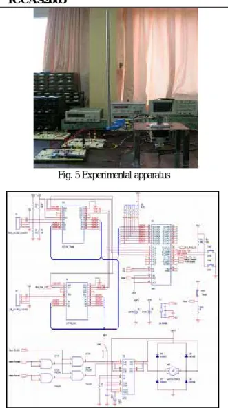
004 . 0 ), 0 , 0 , 0 , 8 , 025 . 0 ( − − − − = = = K R diag Q

Fig. 5 shows pendulum inverted. Fig. 6 is a circuits diagramon which two LS7166 are placed to measure the angles.

(4)

Fig. 5 Experimental apparatus

Fig. 6 Circuits diagram

6. CONCLUSION

Digital deadbeat controller is applied to argumented system. Controllers consist of feedforward integral compensator and local feedback compensator. Especially inverted pendulum has two unstable poles and so these unstable poles are relocated to LHP by pole placement algorithm.

By using conventional digital control design methods, CDBC is easily designed. By comparing simulation it’s well demonstrated, but experiments with SwingUP plus LQR is completed and replacing LQR with CDBC has been doing.

REFERENCE

[1] Ryoichi K. , " Design of Continuous Deadbeat Control, " Tr-SICE, Vol. 28, No.6, pp680-689, 1992.

[2] Eitaku N. , Seiichi S. and Toshiyuki K., " Design of Continuous Deadbeat Tracking Ssytems," Tr-SICE, Vol.28, No.10, p1201-1208, 1992.

[3] E. Nobuyama et. al., "Design of Continuous Deadbeat Tracking Systems," T-SICE, Vol.28, No.10, pp1201 -1208, 1992

[4] Hiroshi M. and Yoshiharu H. ," A Design Method of Continuous Deadbeat Control System," T. IEE Japan, Vol.117-C, No.8, pp.1107- 1112, 1997.

[5] Ryouta S. and Hiroshi M., " A Design Method of Optimal Deadbeat Servosystem and Regulator," T. IEE Japan, Vol.117-C, No.2, pp.117-127, 1997.

[6] Hiroshi M. et. al. " Design of Deadbeat Controller by Using Serial Feedback Compensation," T-SICE, Vol 20, No. 10, pp873-879,1984.

[7] Hiroshi M. et. al. ," Design of Optimal Deadbeat Controller by Using State Feedback," T. IEE Japan, Vol. 109, No. 6, pp.432 - 438, 1996.

[8] Mitsuru O., Yumi. O, Shinichiro. W. and Hiroshi M, "A Design Method of Optimal Continuous Deadbeat Controller by Using Second Delay Element," T. IEE Japan, Vol.118-C, No.5, pp765-772, 1998.

[9] Astrom, K.J. and K. Furuta."Swinging Up A pendulum By Energy Control." IFAC 13th. World Congress, San Francisco, California. 1996.