www.nature.com/scientificreports
Deep learning-based optical
field screening for robust optical
diffraction tomography
DongHun Ryu
1,2, YoungJu Jo
1,2,3,5, Jihyeong Yoo
3, Taean Chang
1,2, Daewoong Ahn
3,
Young Seo Kim
1,2,3,4, Geon Kim
1,2, Hyun-Seok Min
3& YongKeun Park
1,2,3*In tomographic reconstruction, the image quality of the reconstructed images can be significantly degraded by defects in the measured two-dimensional (2D) raw image data. Despite the importance of screening defective 2D images for robust tomographic reconstruction, manual inspection and rule-based automation suffer from low-throughput and insufficient accuracy, respectively. Here, we present deep learning-enabled quality control for holographic data to produce robust and high-throughput optical diffraction tomography (ODT). The key idea is to distil the knowledge of an expert into a deep convolutional neural network. We built an extensive database of optical field images with clean/ noisy annotations, and then trained a binary-classification network based upon the data. The trained network outperformed visual inspection by non-expert users and a widely used rule-based algorithm, with >90% test accuracy. Subsequently, we confirmed that the superior screening performance significantly improved the tomogram quality. To further confirm the trained model’s performance and generalisability, we evaluated it on unseen biological cell data obtained with a setup that was not used to generate the training dataset. Lastly, we interpreted the trained model using various visualisation techniques that provided the saliency map underlying each model inference. We envision the proposed network would a powerful lightweight module in the tomographic reconstruction pipeline.
Quantitative phase imaging (QPI) has played a rapidly expanding role in biomedical applications, due to its label-free, quantitative live-cell imaging capability1. Combined with improved optical designs and computa-tional algorithms, QPI can be expanded to advanced imaging modalities, such as synthetic aperture imaging2, Fourier ptychography3, and tomographic QPI4–6. Amongst them, optical diffraction tomography (ODT) is a three-dimensional (3D) QPI technique that reconstructs a 3D refractive-index (RI) tomogram, based on the Fourier diffraction theorem, from multiple 2D optical fields measured with various illuminations4,7. Thus, the precise acquisition of the multiple 2D images is crucial for tomographic reconstruction. However, undesired noises can be added to the input fields, which deteriorate the image quality of the RI tomograms as they pass through the multiple stages of the ODT reconstruction pipeline (i.e., from hologram acquisition to field retrieval, along with phase wrapping to tomographic reconstruction).
A number of obstacles to robust tomographic reconstruction exist in practice. First, the spectral instability in laser perturbs the interference signals on holograms8. A small shift in the wavelength of the light source can result in substantial changes to the optical path length, thereby generating unintended interference patterns. Second, an illumination control unit, e.g., a digital micromirror device (DMD), may generate unwanted diffraction patterns on the holograms6,9. Third, phase-unwrapping algorithms may fail to operate, thereby generating severe artifects, including phase discontinuity10. An unexpected diffraction of the light passing through a sample, typically arising from dust particles or air bubbles inside the media, can result in abrupt changes in the detected hologram image. These high-gradient signals could cause the phase-unwrapping solver to obtain inaccurate solutions. To prevent possible degradation of the recovered tomogram quality, one can ‘manually’ exclude the noisy fields by eye, and utilise the remaining clean optical fields for the ODT reconstruction. To the best of our knowledge, no rigorous metrics for assessing the retrieved fields in ODT have been investigated while consistent and simple defects could 1Department of Physics, Korea Advanced Institute of Science and Technology (KAIST), 34141, Daejeon, Republic of Korea. 2KAIST Institute for Health Science and Technology, 34141, Daejeon, Republic of Korea. 3Tomocube, Inc., 34109, Daejoen, Republic of Korea. 4Department of Chemical and Biomolecular Engineering, KAIST, 34141, Daejeon, Republic of Korea. 5Present address: Department of Applied Physics, Stanford University, Stanford, CA, 94305, USA. *email: [email protected]
be identified through spatial frequency analysis11. Furthermore, we believe it would be challenging to establish a rule-based metric that considers human perceptive assessment.
To build an effective framework for screening optical fields for robust tomographic reconstruction, consider-ing the above, it is beneficial to employ data-driven approaches, e.g., machine learnconsider-ing and deep learnconsider-ing. With proper data preprocessing and annotation, these approaches can construct a powerful computational model for a wide variety of functions, by learning complex patterns from high dimensional data12. In particular, optical imaging, which deals with a tremendous number of pixels/voxels, has recently been taking full advantage of the data-driven approach13. Synergetic examples include image classification14–18, segmentation19,20, resolution enhancement21,22, noise reduction23,24, light scattering25–27, and in-silico labeling28–30.
Here, we present a deep learning (DL)–based classification network that screens out noisy optical fields for improved tomographic reconstruction. Our network was trained using the classification standard of an ODT expert who annotated large datasets of individual bacteria. For verification, we compared our network with manual classification blinded to the training dataset on the test bacteria dataset, as the network aims for near-human-level classification performance. A rule-based classification algorithm, which computes the peak fre-quency signal of an optical field, was also compared to our method. To assess the generalisability of our method, we classified the optical fields of unseen NIH3T3 cells obtained from a different setup, and reconstructed a tomo-gram from the classified fields, which we then compared with the rule-based algorithm. Finally, we provided three different saliency maps that visualized the network’s inference rationale, which could further validate our data-driven approach.
Methods
Optical diffraction tomography and screening of retrieved optical fields.
The 3D RI tomogram of a sample was reconstructed from multiple 2D holograms, captured with variable-angle illuminations, based on the Fourier diffraction theorem as shown in Fig. 1. Mach-Zehnder interferometry was used for the hologram measurements, and a digital micromirror device (DMD) was utilised for systematic and rapid control of the illumination field9,31. From the 71 measured holograms, corresponding optical fields were retrieved via a field-re-trieval algorithm32. Then, optical fields having unwanted defects, due to the various sources explained above, were sorted out, to improve the image quality of the reconstructed tomogram. In Fig. 1C, 54 clean and 17 noisy optical fields were manually screened. While the clean optical fields of Escherichia coli are clearly shown, the strong fringe patterns and broken optical fields degrade the image quality.Two 3D RI maps were reconstructed from the two sets of input optical fields. The RI tomogram, which was reconstructed from all 71 measured fields (Fig. 1D), contains fringe patterns and ringing artefacts, which, in contrast, are not shown in the recovered tomogram that only uses the clean optical fields after the annotation Figure 1. (A) In ODT, a sample is illuminated from various angles. (B) Holograms obtained under various illumination angles. (C) Optical fields reconstructed from the holograms, including 54 clean and 17 noisy fields annotated by a trained ODT user. (D,E) RI tomograms of E. coli, recovered using all 71 fields and only the 54 clean fields, respectively. (F) Annotation standard. A trained individual has annotated the optical field data to prepare the training and test datasets. (Top) a bacteria cell is visible in the clean background. (Middle) strong unwanted fringe patterns overwhelm the sample, making it hard to identify. (Bottom) the optical fields are totally broken, since unwanted noise was captured in the hologram intensity or no signals were obtained.
www.nature.com/scientificreports
www.nature.com/scientificreports/
(Fig. 1E). Again, these visualisations signify that classifying retrieved optical fields and sorting them are essential in ODT reconstruction. Note that we did not use any regularisation techniques, commonly utilised for addressing the missing-cone problem, to obtain an objective comparison of the image quality33. For the NIH3T3 test dataset used for the generalisation test, we measured a tomogram of cells from a different ODT system, where the setup configuration was identical to the system used for bacterium imaging, except for the number of illumination angles (=45), and the manufacturers of a few optical components. The details of the imaging system are explained in Fig. S1.
Sample preparation.
The 3D RI tomograms of bacteria were acquired from specimens of E.coli, K.pneumo-niae, P. aeruginosa, and S. epidermidis which were cultured in laboratory. The frozen glycerol stocks of bacteria,
stored at −80 °C, were thawed at room temperature. The bacteria were isolated from the glycerol solution by repetitions of centrifugation and washing with fresh media. After stabilization at 35 °C incubator, the bacteria were streaked on agar plates. The agar plates were incubated in 35 °C until colony formation was visible with naked eyes. Single colonies were seeded on fresh media using sterile loops. Each subculture was incubated at a 35 °C shaking incubator until the concentration reached approximately 108–109 cfu/ml. The grown subculture was repeatedly centrifuged and washed, once with fresh medium and twice with phosphate buffered saline (PBS) solution. Finally, the washed bacteria solution was diluted with PBS solution until the concentration was adequate for single-specimen imaging.
The NIH3T3 cells (CCL-2, ATCC, Manassas, VA, USA) were preserved in Dulbecco’s modified Eagle’s medium (DMEM; Life Technologies) containing 100 U/mL streptomycin in humidified air (10% CO2), 10% (vol/ vol) fetal bovine serum (FBS; Gibco, Gaithersburg, MD, USA), and 100 U/mL penicillin at 37 °C.
Data annotation.
The total number of reconstructed optical fields of four species of bacterium (E. coli,Klebsiella pneumoniae, Pseudomonas aeruginosa, and Staphylococcus epidermidis) is 30,814. We imaged 434 RI
tomograms; 71 optical fields were measured to reconstruct each tomogram.
Next, an ODT expert annotated the 30,814 complex fields, according to three types of optical field: one clean and two noisy, as depicted in Fig. 1F. The recovered optical field was labeled as clean if a specimen was clearly visible and the background did not have significant defects. The first noisy-image case was corrupted with strong fringe patterns, emerging from unwanted interference signals. The second noisy-image case included broken images, due to the failure of the phase-unwrapping algorithm. This case typically occurred when the high-angle incident beam was diffracted by dust particles or bubbles in the sample medium, thereby blocking the sample signal at the detector. Both cases hindered the identification of the specimen of interest.
After balancing the two annotated datasets to have an equal number of images (=2,660), we separated the obtained fields into 3,990 and 1,330 images, as training and test datasets, respectively. The NIH3T3 cells were annotated under the same standard. The test sets were never reviewed before the classification network was com-pletely trained.
Deep neural network implementation.
The convolutional neural network, designed for classifying input optical fields in the ODT reconstruction, is illustrated in Fig. 2. For training, we used a single-channel phase image (1 × 128 × 128) as an input to the network, because we observed that the phase image provides higher accuracy than a double-channel complex field (2 × 128 × 128) that concatenates the amplitude and phase, or a single-channel amplitude (See Appendix B).The network architecture consists of two main functional blocks: feature extraction (C1–6) and classification (L1–3). The first block extracts various features using convolutional filters and non-linearity. The 1 × 128 × 128 Figure 2. Architecture of the deep neural network for classifying optical fields in ODT. The feature extraction part, composed of the convolution layer, ReLu (Rectified Linear Unit), max pooling, and adaptive max pooling, generates 1,024 feature maps. They are converted into a single scalar in the classification part for the final inference. C and L stand for convolutional block and linear block, respectively. n is the image dimension and p is the dropout rate.
input images are processed to become 512 4×4-feature images, after passing through five consecutive sub-blocks consisting of a convolutional filter (the number of filters doubles in each sub-block (32, 64, 128, 256, and 512), rectified non-linearity (ReLu), and max pooling (slide = 2). Then, at the last C6, with the convolution, ReLu, and adaptive max pooling forcing it to have a single scalar output, 1,024 feature maps are generated before entering the fully connected layers for the classification.
The following three sub-blocks (L1−3), consisting of a dropout layer (p = 0.3, 0.5, and 0.5), a linear layer (1024-512-512-1), and a final sigmoid function (equation), shrink the 1,024 feature maps to a single scalar [0, 1]. This is used to infer whether the input image is defective or clean, given a threshold that can be tuned between 0 and 1. Here, we chose 0.5 for the threshold, based on the network performance.
The deep-learning model was implemented in a Pytorch 0.3.1 framework using a GPU server (two Intel
®
Xeon®
CPUs E5-2620 v4, eight NVIDIA GeForce GTX 1080 Ti, and 11 GB memory). We center-cropped each image to 128 × 128 pixels, and carried out an elastic transform34, which is widely used in data augmentation to accelerate network performance. We used an ADAM optimiser35 and binary cross-entropy as the loss function to train the network. Typical training-epoch numbers range from 5 to 30 to achieve over 90% accuracy. We heu-ristically stopped the algorithm at epoch 20. For the single-channel phase dataset, the averaged training time for 10 different random initialisations was approximately 20 minutes with a batch size of 16. Typically, the time com-plexity of the convolutional neural network is “linearly” proportional to the size of the input (i.e., the number of voxels), the number of parameters, and the size of each hidden layers. Although the training time heavily depends on the batch size, the number of GPUs and epoch numbers, training our suggested simple network with larger image sizes (256 × 256–512 × 512) can be achieved within 2–3 hours. We employed He’s initialisation36, which considers the rectifiers as nonlinearities, for the convolutional layers, and Xavier’s initialisation37 for the linear layers. We can classify an arbitrary input image in real time, once the network is trained.Blind evaluations.
Five physicists with novice levels of ODT experience evaluated the pre-split test data of bacteria optical fields for comparison with our method. While the annotator has more than three years of experi-ences with QPI technologies, including ODT, all the participants for the blind evaluations have less than one-year experience. The test data were split into five sets, consisting of 200 images without repetition, and given to the raters. Note that the physicists were neither involved in the data acquisition nor exposed to the initial annotating process.Rule-based algorithm for classifying optical fields.
To benchmark the proposed classification net-work, we implemented a rule-based algorithm exploiting the peak signal of a given optical field in Fourier space. Because most biological samples are transparent (weakly scattered), low spatial-frequency components are dom-inant in the captured optical fields. By contrast, strong fringe patterns or abrupt phase changes could generate abnormally high values in the high spatial-frequency information (Fig. 3, left).We also outline the procedure for the rule-based classification algorithm (Fig. 3, right). For each 2D optical field, we first compute the absolute spectrum (in log10) of the spatial Fourier transform. Second, the peak values outside a user-specified high-pass mask, centered at the illumination wave vector (i.e., sam-ple low-spatial-frequency component), were used to screen the fields. To ensure that we focus on the high spatial-frequency region, the mask size was chosen to be large enough to occlude the low-spatial-frequency com-ponent. Here, we chose 40 × (1/0.16) (μm−1) as a mask diameter. Then, optical fields in which the peak value exceeded a user-specified threshold were classified to reconstruct a RI tomogram. For the screening threshold value, we heuristically chose 2.705 and 3.306 to screen the bacteria and NIH3T3 optical fields, respectively. Note Figure 3. Rule-based algorithm for classifying optical fields. (Left) clean and noisy NIH3T3 phase images and their Fourier spectrum. (Right) flowchart/procedure of the algorithm that computes the peak value of the high-frequency region for each optical field.
www.nature.com/scientificreports
www.nature.com/scientificreports/
that the valuye in the range of 2−4 has been found as an optimal range of thresholding values based on our exten-sive work of labelling optical fields.
Deep learning visualisation methods.
Three visualisation techniques were utilized to elucidate the spatial distributions of the image-activation map that led to our deep network’s decision: class activation mapping (CAM), guided back propagation (Guided BP), and gradient-weighted class activation mapping (Grad-CAM), which all are described in more detail elsewhere38–40. All of these methods use localisation maps, which conserve the spatial information of the network input in convolutional layers and expand them to an input-sized saliency map.The CAM images illustrated below (see Results and Discussion) are generated at the last convolutional layer (C6 in Fig. 2) before entering the classification layers (L1−3). The guided BP images are generated at the end of C2. They are bilinearly upsampled to the dimension of the network input to clearly visualise the saliency-map distribution that our algorithm might have used for inference. Lastly, Grad-CAM images are created via the point-wise product CAM and guided BP products.
Result
Training of DL-based classification network.
We first trained a neural network for the binary classifica-tion of optical fields using datasets consisting of four classes of bacterium (E. coli, K. pneumoniae, P. aeruginosa, and S. epidermidis). The convolutional neural network that determines whether a given optical field is clean or noisy was trained using gradient descent–based optimisation and stopped with epoch 20, when the validation accuracy typically started to decrease in our algorithm (see Methods for details). Here, we present the averaged training and test accuracy for 10 different initialisations of model weights. The training accuracy of the network achieved 98.97 ± 0.68% (±standard deviation, SD). Specifically, the accuracies for the clean images (sensitivity) and noisy images (specificity) are 98.86 ± 0.97% and 99.09 ± 0.74%, respectively.Classification results of the network.
To test the performance of the trained network in terms of accu-racy, we compared our proposed method with a classification that was screened by five human raters who had not seen the dataset, and a rule-based algorithm that computes a maximum value in the high-frequency region of Fourier space (Fig. 4, see also Methods). For the bacteria test data, the proposed method achieved 92.15 ± 0.07%, outperforming the averaged accuracy of the five human raters’ classification, 76.22 ± 4.11%, and the rule-based algorithm, 65.71%, (Fig. 4A) To study how much of each image class is correctly classified, the specificity (clean) and sensitivity (noisy) of the three methods are shown in Fig. 4B. The proposed classification network obtained higher test accuracy: proposed method (92.28 ± 3.06% and 92.35 ± 2.57%), human raters (72.51 ± 9.19% and 79.93 ± 5.22%), and rule-based algorithm (95.94% and 35.49%).To investigate whether the surpassing test accuracy of the present method results in improved tomograms, we reconstructed three RI tomograms of E. coli from the three screened optical-field sets. The reconstructed images from the present method and the rater who achieved the best accuracy have fewer artefacts in the background, in comparison to the rule-based algorithm. We also measured the SD of the boxed region for the Figure 4. Performance of deep learning, human raters, and rule-based algorithm on the field classification, and corresponding tomogram reconstructions. (A) Total training and test accuracy are compared for the present and three other methods. (B) For each case in (A), the specificity and sensitivity of two classes (clean and noisy) are investigated. (C) 2D sliced images of 3D tomograms are compared, and background noises are quantified via the standard deviation computed in the shaded region.
three reconstructed tomograms. The SDs of the present method, human raters, and rule-based algorithm are 0.91×10⁻³%, 0.90×10⁻³%, and 1.60×10⁻³%, respectively (Fig. 4C).
Three remarks on this comparative study are noteworthy. First, while the test accuracies of the raters are approximately 16% lower than those of our method (Fig. 4A), their reconstructed image qualities and noise levels are not notably distinguishable. This seems to be because the raters and our classification network that learned expert perception are capable of sorting out noisy optical fields that would significantly deteriorate the recon-structed tomogram, which may not be screened by the naïve algorithm introduced here. Second, the standard deviations of the accuracies for the human raters are greater than those of the deep learning, which implies that the manual screening may not return a consistent output. Third, the image qualities (e.g., visibility of E. coli) of the reconstructed tomograms are not notably different, although the three optical-field datasets have a different num-ber of angle illuminations. To some extent, the reduced numnum-ber of illuminations in ODT can provide a reasonable quality of tomogram output, which has been more systematically investigated elsewhere41,42.
Generalisation test on noisy eukaryotic cell.
To further examine the proposed method in a worse-case scenario and its generalisability, we imaged eukaryotic cells (NIH3T3) using an ODT imaging system that was not used to obtain the training set, as depicted in Fig. 5. Note that we chose the optical-field set that contained more noisy images than clean images for this test (22 clean and 23 noisy images). We first used 22 clean optical fields to reconstruct 3D tomograms, which were used as a gold standard to evaluate our method and the rule-based algo-rithm. Figure 5A,B display reconstructed tomograms using all 45 optical fields, and using only the 22 clean fields as the ground truth, respectively. They visualise the significance of field screening in tomographic reconstruction.In Fig. 5C,D, our classification network generated a reconstructed tomogram with a similar quality level as the gold standard, in contrast to the poorly reconstructed tomogram using the rule-based algorithm. The total classification accuracy, specificity (clean), and sensitivity (noisy) of our method are 84.44%, 72.72%, and 95.65%, respectively; the accuracies of the rule-based algorithm for the same cases are 65.71%, 95.94%, and 35.49%, respectively. Including noisy fields in the reconstruction severely degrades the image quality of the RI tomogram, though the specificity (i.e., accuracy for clean fields) of the rule-based algorithm exceeds that of our method. This finding reemphasizes that screening optical fields in the ODT reconstruction is a critical process to determine the image quality of reconstructed tomograms. As the last remark, other rule-based algorithms using differ-ent metrics, such as image gradidiffer-ent and image statistics (e.g., max, min, mean, and standard deviation), could be employed to improve the field classification particularly for these type of critical noises (See Supplementary Information). However, fine-tuning of algorithmic parameter, based on given data distribution, should be carried out to yield improved screening performance.
Visualisation of network inference toward interpretable deep learning.
To interpret the results, we obtained saliency maps that highlighted the spatial regions relevant to the network inference, using Figure 5. Generalisation test: NIH3T3 cell tomograms (sliced at axial center, Δ z = 0 μm) are recovered from various classified optical field data from (A) all 45 fields, (B) ground truth prepared by the expert, (C) the rule-based algorithm, and (D) the present method. (E) 3D iso-surface rendering of the tomogram recovered from the ground-truth optical fields. (F) The specificity and sensitivity, along with the total test accuracy, are depicted.www.nature.com/scientificreports
www.nature.com/scientificreports/
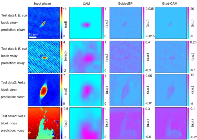
three widely used visualisation techniques (see Methods). For the four types of image (clean/noisy E. coli and clean/noisy NIH3T3), the input phase image, corresponding class activation mapping (CAM) images, guided back-propagation (GuidedBP) images, and gradient-weighted class activation mapping (Grad-CAM) images are depicted in Fig. 6 (columns 1−4). The CAM images do not display the details of the interesting objects (i.e., E.
coli, NIH3T3), but distinguish the objects from the background. Unlike the CAM images, the BP images provide
a global distribution of the activations with a higher resolution; however, the information around the specimens is less localised. Finally, the Grad-CAM images, inferred as clean (rows 1 and 3), elucidate a more localised detection of the target specimen, while parasitic fringe patterns and broken phases, dispersed across the images, are visible in the noisy images (rows 2 and 4). These saliency maps well represent the decision-making process of the algo-rithm, as one could look through the overall image and detect the object boundary or any defects in the image.
Discussion
We proposed and experimentally demonstrated a deep neural network that screens optical fields to improve the image quality of RI tomograms in ODT. The proposed network, trained with an optical-field dataset annotated by a human expert, outperformed the overall classification results produced by human raters and the rule-based algorithm by a large margin (>20%). To understand the inner workings of our model beyond its results, we uti-lised various visualisation techniques to obtain saliency maps that highlight the pixels relevant to the predictions. We envision that the proposed classification framework, replacing the perception of the well-trained experimen-talist, would enable a fast, automated, and consistent tomographic reconstruction, which is possible for ODT and can be extended to tomographic-reconstruction methods in general.
Additional improvement aspects can be investigated to supplement our classification network. The present annotation standard can be further systematically established, rather than manually classifying input optical fields into three categories (clean, fringe noise, and broken-image noise). We relied entirely on the visual perception of the experienced ODT expert, to make the qualitative ground-truth label for the dataset. Reconstructing a test sample with a known RI from various optical-field combinations may provide a quantitative method for select-ing input fields to improve the reconstructed tomograms. Furthermore, a large number of annotators can make a better gold standard, which would enable the artificial intelligence (AI) model to learn from their collective intelligence.
Figure 6. Visual interpretations of the deep network inference. For each class (clean and noisy) of the phase image for E. coli and NIH3T3 (column 1), we extracted a class activation mapping image (CAM) (column 2), guided back-propagation (GuidedBP) (column 3), and gradient-weighted class activation mapping (Grad-CAM) (column 4). Among the three visualization techniques, the Grad-CAM images, generated from the point-wise product of CAM and guided BP, best display the anatomical region that our deep neural network might have utilized for its inference.
On the other hand, image detection and classification problems can establish a gold standard for most cases, which can be very reliable domains for deep-learning technology. We believe that various problems in imag-ing science, particularly those related to image classification, can continue to leverage AI technologies to aid or replace the tremendous amount of laborious work.
Data availability
All data sets and code packages will be available after the underway commercialisation of this work. Received: 17 April 2019; Accepted: 27 September 2019;
Published: xx xx xxxx
References
1. Park, Y., Depeursinge, C. & Popescu, G. Quantitative phase imaging in biomedicine. Nat. Photonics 12, 578–589, https://doi. org/10.1038/s41566-018-0253-x (2018).
2. Ralston, T. S., Marks, D. L., Carney, P. S. & Boppart, S. A. Interferometric synthetic aperture microscopy. Nat. Phys. 3, 129 (2007). 3. Zheng, G., Horstmeyer, R. & Yang, C. Wide-field, high-resolution Fourier ptychographic microscopy. Nat. Photonics 7, 739 (2013). 4. Wolf, E. Three-dimensional structure determination of semi-transparent objects from holographic data. Opt. Comm. 1, 153–156
(1969).
5. Kim, T. et al. White-light diffraction tomography of unlabelled live cells. Nat. Photonics 8, 256 (2014). 6. Cotte, Y. et al. Marker-free phase nanoscopy. Nat. Photonics 7, 113 (2013).
7. Kim, K. et al. Optical diffraction tomography techniques for the study of cell pathophysiology. 2 (2016).
8. Lee, K., Shin, S., Yaqoob, Z., So, P. T. & Park, Y. Low-coherent optical diffraction tomography by angle-scanning illumination. arXiv
preprint, arXiv:1807.05677 (2018).
9. Shin, S., Kim, K., Yoon, J. & Park, Y. Active illumination using a digital micromirror device for quantitative phase imaging. Opt.
Express 40, 5407–5410 (2015).
10. Pritt, M. D. & Ghiglia, D. C. Two-dimensional phase unwrapping: theory, algorithms, and software. (Wiley, 1998).
11. Ajithaprasad, S., Velpula, R. & Gannavarpu, R. Defect detection using windowed Fourier spectrum analysis in diffraction phase microscopy. Journal of Physics Communications 3, 025006 (2019).
12. LeCun, Y., Bengio, Y. & Hinton, G. Deep learning. Nature 521, 436 (2015).
13. Jo, Y. et al. Quantitative Phase Imaging and Artificial Intelligence: A Review. IEEE J. of Sel. Top. in Quantum Electron. 25, 1–14,
https://doi.org/10.1109/JSTQE.2018.2859234 (2019).
14. Nguyen, T. H. et al. Automatic Gleason grading of prostate cancer using quantitative phase imaging and machine learning. J.
Biomed. Opt. 22, 036015 (2017).
15. Rawat, S., Komatsu, S., Markman, A., Anand, A. & Javidi, B. Compact and field-portable 3D printed shearing digital holographic microscope for automated cell identification. Appl. Opt. 56, D127–D133 (2017).
16. Jo, Y. et al. Holographic deep learning for rapid optical screening of anthrax spores. Sci. Adv. 3, e1700606 (2017).
17. Yoon, J. et al. Label-Free Identification of Lymphocyte Subtypes Using Three-Dimensional Quantitative Phase Imaging and Machine Learning. JoVE, e58305, https://doi.org/10.3791/58305 (2018).
18. Kim, G., Jo, Y., Cho, H., Min, H.-S. & Park, Y. Learning-based screening of hematologic disorders using quantitative phase imaging of individual red blood cells. Biosens. Bioelectron. 123, 69–76 (2019).
19. De Fauw, J. et al. Clinically applicable deep learning for diagnosis and referral in retinal disease. Nat. Med. 24, 1342 (2018). 20. Lee, J. et al. Deep-learning-based label-free segmentation of cell nuclei in time-lapse refractive index tomograms. BioRxiv, 478925
(2018).
21. Nehme, E., Weiss, L. E., Michaeli, T. & Shechtman, Y. Deep-STORM: super-resolution single-molecule microscopy by deep learning.
Optica 5, 458–464 (2018).
22. Nguyen, T., Xue, Y., Li, Y., Tian, L. & Nehmetallah, G. Deep learning approach for Fourier ptychography microscopy. Opt. Express
26, 26470–26484, https://doi.org/10.1364/OE.26.026470 (2018).
23. Choi, G. et al. Cycle-consistent deep learning approach to coherent noise reduction in optical diffraction tomography. Opt. Express
27, 4927–4943 (2019).
24. Jeon, W., Jeong, W., Son, K. & Yang, H. Speckle noise reduction for digital holographic images using multi-scale convolutional neural networks. Opt. Lett. 43, 4240–4243, https://doi.org/10.1364/OL.43.004240 (2018).
25. Li, S., Deng, M., Lee, J., Sinha, A. & Barbastathis, G. Imaging through glass diffusers using densely connected convolutional networks. Optica 5, 803–813 (2018).
26. Li, Y., Xue, Y. & Tian, L. Deep speckle correlation: a deep learning approach toward scalable imaging through scattering media.
Optica 5, 1181–1190 (2018).
27. Rahmani, B., Loterie, D., Konstantinou, G., Psaltis, D. & Moser, C. Multimode optical fiber transmission with a deep learning network. Light Sci. Appl. 7, 69, https://doi.org/10.1038/s41377-018-0074-1 (2018).
28. Christiansen, E. M. et al. In silico labeling: Predicting fluorescent labels in unlabeled images. Cell 173, 792–803 (2018).
29. Ounkomol, C., Seshamani, S., Maleckar, M. M., Collman, F. & Johnson, G. R. Label-free prediction of three-dimensional fluorescence images from transmitted-light microscopy. Nat. Methods 15, 917 (2018).
www.nature.com/scientificreports
www.nature.com/scientificreports/
30. Rivenson, Y. et al. Deep learning-based virtual histology staining using auto-fluorescence of label-free tissue. arXiv preprint
arXiv:1803.11293 (2018).
31. Lee, K., Kim, K., Kim, G., Shin, S. & Park, Y. Time-multiplexed structured illumination using a DMD for optical diffraction tomography. Opt. Express 42, 999–1002 (2017).
32. Takeda, M., Ina, H. & Kobayashi, S. Fourier-transform method of fringe-pattern analysis for computer-based topography and interferometry. JOSA A 72, 156–160 (1982).
33. Lim, J. et al. Comparative study of iterative reconstruction algorithms for missing cone problems in optical diffraction tomography.
Opt. Express 23, 16933–16948 (2015).
34. Jaderberg, M., Simonyan, K. & Zisserman, A. In Adv. Neural Inf. Process. Syst. 2017–2025 (2015). 35. Kingma, D. P. & Ba, J. Adam: A method for stochastic optimization. arXiv preprint, arXiv:1412.6980 (2014). 36. He, K., Zhang, X., Ren, S. & Sun, J. In Proc. IEEE Int. Conf. Comput. Vis. 1026–1034 (2015).
37. Glorot, X. & Bengio, Y. In Proceedings of AISTATS 2010. 249–256 (2010).
38. Springenberg, J. T., Dosovitskiy, A., Brox, T. & Riedmiller, M. Striving for simplicity: The all convolutional net. arXiv preprint,
arXiv:1412.6806 (2014).
39. Zhou, B., Khosla, A., Lapedriza, A., Oliva, A. & Torralba, A. In Proc. IEEE Comput. Soc. Conf. Comput. Vis. Pattern Recognit. 2921–2929 (2015).
40. Selvaraju, R. R. et al. In Proc. IEEE Int. Conf. Comput. Vis. 618–626 (2016).
41. LaRoque, S. J., Sidky, E. Y. & Pan, X. Accurate image reconstruction from few-view and limited-angle data in diffraction tomography.
JOSA A 25, 1772–1782 (2008).
42. Kim, K., Kim, K. S., Park, H., Ye, J. C. & Park, Y. Real-time visualization of 3-D dynamic microscopic objects using optical diffraction tomography. Opt. Express 21, 32269–32278 (2013).
43. Adebayo, J. et al. In Adv. Neural Inf. Process. Syst. 9525–9536 (2018).
44. Jiang, H., Kim, B., Guan, M. & Gupta, M. In Adv. Neural Inf. Process. Syst. 5546–5557 (2018).
45. Yeh, C.-K., Hsieh, C.-Y., Suggala, A. S., Inouye, D. & Ravikumar, P. How Sensitive are Sensitivity-Based Explanations? arXiv preprint,
arXiv:1901.09392 (2019).
Acknowledgements
This work was supported by KAIST, Tomocube, and National Research Foundation of Korea (2015R1A32066550, 2017M3C1A3013923, 2018K000396).
Author contributions
D.H.R., Y.J.J. and Y.K.P. designed the project. D.H.R. implemented the deep learning algorithm with the help of J. Y. and D.A.. D.H.R., Y.J.J., Y.S.K., H.-S.M. and Y.K.P analyzed the results. T.C. and G.K. provided the datasets. All authors wrote the manuscript.
Competing interests
Mr. Yoo, Mr. Ahn, Mr. Kim, Dr. Min, and Prof. Park have financial interests in Tomocube Inc., a company that commercializes ODT and is one of the sponsors of the work.
Additional information
Supplementary information is available for this paper at https://doi.org/10.1038/s41598-019-51363-x. Correspondence and requests for materials should be addressed to Y.P.
Reprints and permissions information is available at www.nature.com/reprints.
Publisher’s note Springer Nature remains neutral with regard to jurisdictional claims in published maps and institutional affiliations.
Open Access This article is licensed under a Creative Commons Attribution 4.0 International License, which permits use, sharing, adaptation, distribution and reproduction in any medium or format, as long as you give appropriate credit to the original author(s) and the source, provide a link to the Cre-ative Commons license, and indicate if changes were made. The images or other third party material in this article are included in the article’s Creative Commons license, unless indicated otherwise in a credit line to the material. If material is not included in the article’s Creative Commons license and your intended use is not per-mitted by statutory regulation or exceeds the perper-mitted use, you will need to obtain permission directly from the copyright holder. To view a copy of this license, visit http://creativecommons.org/licenses/by/4.0/.