저작자표시-비영리-변경금지 2.0 대한민국 이용자는 아래의 조건을 따르는 경우에 한하여 자유롭게 l 이 저작물을 복제, 배포, 전송, 전시, 공연 및 방송할 수 있습니다. 다음과 같은 조건을 따라야 합니다: l 귀하는, 이 저작물의 재이용이나 배포의 경우, 이 저작물에 적용된 이용허락조건 을 명확하게 나타내어야 합니다. l 저작권자로부터 별도의 허가를 받으면 이러한 조건들은 적용되지 않습니다. 저작권법에 따른 이용자의 권리는 위의 내용에 의하여 영향을 받지 않습니다. 이것은 이용허락규약(Legal Code)을 이해하기 쉽게 요약한 것입니다. Disclaimer 저작자표시. 귀하는 원저작자를 표시하여야 합니다. 비영리. 귀하는 이 저작물을 영리 목적으로 이용할 수 없습니다. 변경금지. 귀하는 이 저작물을 개작, 변형 또는 가공할 수 없습니다.
Master’s Thesis of Forest Sciences
Thirty-two years of Mangrove Forest
Land Cover Change in Parita Bay,
Panama
파나마 Parita Bay에서 32 년간의 맹그로브 숲 토지
피복 변화
August 2019
Graduate School of Agriculture and Life Science
Seoul National University
Forest Environmental Sciences Major
Yoisy Belen Castillo Gutierrez
i
Abstract
Mangroves forests around the world have been experiencing a drastic loss. This decrease is attributed in part to changes in bio-climatic factors (e.g. rainfall, temperature, tidal range, extreme events, etc.) and to anthropogenic activities such as coastal development, agriculture, timber extraction, upstream discharge of contaminants, as well as aquaculture and saltpan construction. Whereas remote sensing tools have contributed to detect mangrove vulnerable areas in order to respond with appropriate conservation policies. The principal aims of our study are to quantify the changes in mangrove cover and to identify possible drivers of its change. We present the first mangrove land cover-change analysis in Panama using satellite imagery after the year 2000, and the first in Parita Bay. Mangrove cover changes were determined using Landsat satellite images in four (4) points of time: 1987, 1998, 2009 and 2019, which consequently, were subdivided into three (3) period of study. A supervised classification was employed to quantify changes in areas of different land use-cover types; and the NDVI (Normalized Difference Vegetation Index) was determined for each image, in order to observe changes of greenness in mangrove canopy cover. Our study revealed mangrove area in Parita Bay has increased by 4.7% during the last 32 years and seems to have a good health status reflected in the presence of high NDVI values. However, there was a 1.26% decline of mangrove cover at the first period (1987 to 1998), principally related to the conversion into ‘other types of vegetation’ and ‘bare soil’. During the same period, results also revealed a high expansion of aquaculture and saltpan by 95.88%, and a decline of ~40% in high and very high-density NDVI (>0.46). After the initial decrease of mangrove area, it increased 6% of its extent for the last two decades, and the annual increment rate was even greater for the last decade (0.43%). The increase of mangroves in Parita Bay was mostly due to the conversion from ‘water’, ‘other vegetation’ and ‘bare soil’ classes. This leads to assume that natural regeneration characteristics coupled with restoration projects developed in the region may had a positive influence over the mangrove cover. In addition, mangroves in protected areas declined at an annual rate of 0.11%, while the
ii
unprotected mangroves increased at 0.50% per year during the last period (2009-2019). Our study suggests continuous management of mangrove forests is essential for the areas where the ecosystem vulnerability is high.
Keywords: Mangroves, remote sensing, Land use-cover change (LUCC),
Normalized Difference Vegetation Index (NDVI), Landsat, aquaculture, Panama
iii
Table of Content
1. Study Area ... 5
2. Data Selection and Image preprocessing ... 6
3. Image Classification ... 7
4. Field Ground Truth and Accuracy Assessment ... 10
5. NDVI Analysis ... 11
6. Land Cover-Use Change (LUCC) detection ... 12
7. Analysis in Protected Areas ... 13
8. Analysis of Environmental variables in the study area ... 13
1. Classification Accuracy ... 16
2. Land Use-Cover Change (LUCC) Detection and mangrove estimation in Parita Bay ... 18
3. NDVI Classes Changes on time ... 23
5. Mangroves changes in Protected vs. Unprotected Area ... 28
6. Local Climatic Variables Analysis ... 33
6.1 Rainfall ... 33 6.2 Temperature ... 34 Appendix A ... 52 Appendix B ... 54 Appendix C ... 55 Appendix D ... 56
I.
Introduction ... 1
II.
Material and Methods ... 5
III.
Results ... 16
IV.
Conclusion ... 43
References... 45
Web References... 51
Abstract (in Korean) ... 57
iv
List of Tables
Table 1. Data products used for the study ... 7 Table 2. Pixel-based Error Matrix for the classified 2019 Landsat Image. AS= Aquaculture and Saltpans, BB=Bare soil & Built-up... 17 Table 3. Pixel-based Error Matrix for the classified 2009-2010 composite Landsat Image. AS= Aquaculture and Saltpans, BB=Bare soil & Built-up ... 17 Table 4. Land Use-Cover area change and rate of change in Parita Bay from 1987 to 2019. The composite image from 2009-2010, for practical reasons is defined as only 2010 for the Change Analysis. ... 19 Table 5. Matrix of Change for Mangrove Class from 1987 to 2019. Class 1=Mangrove, 2=Water, 3=Aquaculture and Salt-Pans, 4=Other vegetation, and 5=Bare soil and Built-up. ... 20 Table 6 Matrix of Change for AS Class from 1987 to 2019. Class 1=Mangrove, 2=Water, 3=Aquaculture and Saltpans, 4=Other vegetation, and 5=Bare soil and Built-up. ... 21 Table 7. NDVI Density Classes Change between 1987 and 2019 ... 24 Table 8. Land Use-Cover loss and gains in Cenegon de Mangle Wildlife Refuge and Sarigua National Park ... 30 Table 9. Land Use-Cover loss and gains in the unprotected region of the study area ... 30 Table 10. Matrix of Change for Mangrove Class in Cenegon de Mangle from 1987 to 2019. Class 1=Mangrove, 2=Water, 4=Other vegetation, and 5=Bare soil and Built-up. ... 31 Table 11. Matrix of Change for Mangrove Class in Sarigua National Park from 1987 to 2019. Class 1=Mangrove, 2=Water, 3=Aquaculture and Saltpans, 4=Other vegetation, and 5=Bare soil and Built-up. ... 32 Table 12. Accumulative Rainfall (mm) 90 days before each capture ... 34
v
List of Figures
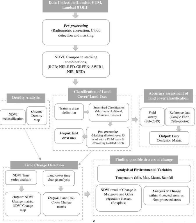
Figure 1. Location of Study Area in Parita Bay, Panama. Source: google maps. ... 6 Figure 2. Flowchart of the study ... 8 Figure 3. Random sampling of 500 pixel points of NDVI values in unchanged mangrove cover. ... 12 Figure 4. Protected Areas located in the study region of Parita Bay. a) Study region Landsat 8 RGB composite raster. b) ‘Cenegon de Mangle’ Wildlife Refuge and ‘Sarigua’ National Park zoomed area. ... 13 Figure 5 View of the Meteorological stations in Parita Bay. Rainfall data was obtained from ‘Rio Hondo’, ‘Puerto Posada’, ‘Parita’ and ‘Los Santos’ stations. Temperature data was obtained from ‘Parita’ and ‘Los Santos’ stations. ... 15 Figure 6. Parita Bay Land Use-Cover classification of the images from 1987, 1998, 2009-2010 and 2019. ... 22 Figure 7. Graphic of Land Cover- Land Use Change in Parita Bay for Mangrove, Aquaculture & Salt-Pans (AS), Other vegetation and Bare soil & Built-up (BB) classes. Water category was excluded. ... 22 Figure 8. Mangrove cover extent (in hectares) in Parita Bay for the years 1987, 1998, 2009-2010 and 2019. ... 23 Figure 9. NDVI Density classes area (ha) changes in the Parita Bay from 1987 to 2019. ... 25 Figure 10. Parita Bay NDVI density map for a) 1987, b)1998, c)2009-2010, and d) 2019. ... 25 Figure 11. Boxplots of Mangrove NDVI samples from 1987 to 2019. . ... 26 Figure 12. Mangrove area change and NDVI trend for each satellite image in Parita Bay. ... 27 Figure 13. Boxplots of Other vegetation NDVI values sampled from 1987 to 2019. ... 28 Figure 14 Cenegon de Mangle Wildlife Refuge and Sarigua National Park extracted Land Use-Cover maps from 1987, 1998, 2009-2010, and 2019 in Parita Bay. ... 29 Figure 15. Comparison of the annual rate of change for both Protected versus Unprotected areas. ... 29
vi
Figure 16. Annual accumulative rainfall in Parita Bay from January 1986 to December 2018. ... 33 Figure 17. Rainfall 3 months before the date of capture of each Landsat imagery. 34 Figure 18. Minimum, Mean and Maximum Temperature in Parita Bay from 1986 to 2019. ... 35 Figure A-1. Mangrove gains and losses during 1987 to 2019 in Parita Bay.52 Figure A-2. Mangrove gains and losses during 1987 to 1998 in Parita Bay. ... 52 Figure A-3. Mangrove gains and losses during 1998 to 2009-2010 in Parita Bay. 53 Figure A-4. Mangrove gains and losses during 2009-2010 to 2019 in Parita Bay.. 53 Figure B-1. Histograms of mangrove cover NDVI (500) samples (skewed left distribution). ... 54 Figure B-2. Histograms of other vegetation cover NDVI (500) samples. ... 54 Figure D-1. ‘Magrove Fern’ (Acrostichum aureum) observed in the Puerto Posada, Cocle Province. ... 56 Figure D-2. Ground Control Points field collection. Back: (Conocarpus Erectus) Bottonwood mangrove. ... 56
1
I.
Introduction
Mangroves comprises the group of halophytic trees, shrubs and plants positioned in the critical interface between terrestrial, estuarine, and near-shore marine ecosystems in the tropical and subtropical coastlines (J. B. Kauffman & Donato, 2012; Polidoro et al., 2010), extending from arid zones to cool-temperate coasts (between latitudes 35N and 38S) (Alatorre et al., 2015; Thomas et al., 2017). There are many studies highlighting the importance of mangrove forest due to the ecosystem services they provide, such as nurseries for marine species, sediment stabilization, water purification, woody and non-woody forest products, conservation of biological diversity, coastal protection, and highest rate of carbon sequestration (Friess, 2016; Godoy, De Andrade Meireles, & De Lacerda, 2018; Rioja-Nieto, Barrera-Falcón, Torres-Irineo, Mendoza-González, & Cuervo-Robayo, 2017). As one of the most effective carbon sink forests, mangrove can contain an average of 937 tC ha-1, promoting
speedy rates of sediment deposit (~5 mm year-1) and carbon burial (174 gC m -2 year-1) (Alongi, 2012). Mangroves forest and its soils can sequester
approximately 22.8 million metric tons of carbon each year worldwide (Giri et al., 2011).
Mangrove area around the world according to World Atlas of Mangrove (Spalding, et al., 2010) is approximately 152,000 km2 within 123 countries, and
comprising 73 species. However, this amount was bigger before. Globally, 20 percent (3.6 million hectares) have been lost from 1980 to 2005; from which Indonesia, Mexico, Pakistan, Papua New Guinea and Panama recorded the largest losses during the 1980s (FAO, 2007). There are numerous threats surrounding these ecosystems, some of the most important includes: human population growth, upstream pollution, timber extraction, land use change, agriculture, coastal development projects, aquaculture shrimp ponds, extreme weather events, sea level rise, as well as changes in precipitation and temperature (Brown, Pearce, Leon, Sidle, & Wilson, 2018; Donato et al., 2011; Gilman, Ellison, Duke, & Field, 2008; Hsu & Lee, 2018; McGowan et al., 2010;
2
Valderrama-Landeros, Flores-de-Santiago, Kovacs, & Flores-Verdugo, 2018). This last one, referring to the effect of climatic variables on the mangrove ecosystem is poorly understood. As Climate Change brings an irregular distribution of rainfall worldwide (Solomon et al., 2007), effects over mangrove forest will vary. For example, increasing rainfall may result in a greater mangrove growth rate. While, decreasing rainfall may alter their survival and growth, leading to a decrease in biodiversity and reduction in mangrove area (Gilman et al., 2008). The issues related to mangroves vulnerability have turned into a serious matter that even scientific community stated mangrove forest may functionally dissapear within 100 years (Duke et al., 2007).
Every study represents a valuable contribution to understand the behavior, resilience, and risks related with the future of mangrove ecosystem. Global Land Cover-Mapping studies looks towards the producing scenarios; while regional studies set the basis and provide the tools for local stakeholders in the decision making regarding land-use changes. (Lambin & Geist, 2006). The information about the location of mangroves destruction is essential to determine where mangrove forests reserves are necessaries, and at the same time to comprehend how is the response to environmental and stressor factors in order to set policies of coastal adaptation, resource consumption, or protected areas (Hu, Li, & Xu, 2018). On the other hand, to monitor mangrove ecosystem by fieldwork is quite complicated due to difficult access, flooded soils, soft sediments, wild animals, and other factors. Consequently, remote sensing have been broadly used to monitor mangrove forests, as it is a reliable alternative to perform extensive ground-survey methods of mapping (Flores-Cárdenas et al., 2018; Valderrama-Landeros et al., 2018). It is a tool that can be use with limited funds through open source softwares and free available satellites imagery, allowing developing countries to monitor changes and to assess the effectiveness or impacts of policies and regulations, as well as other climatic variables on ecosystems. (Gaw, Linkie, & Friess, 2018; Ghosh, Kumar, & Roy, 2017; Godoy, De Andrade Meireles, & De Lacerda, 2018; Mondal, Trzaska, & De Sherbinin, 2018; Nursamsi, 2017; Servino, Gomes, & Bernardino, 2018; and
3
others). In this sense, the purpose of this study is to make use of these remote sensing techniques to determine how mangrove land cover has changed in Parita Bay, Panama.
Panama is situated in the 16th position of the global ranking of largest
mangrove holding nations, with 1,323 km2 (Hamilton & Casey, 2016). Further,
it can be said is the country with the largest mangrove cover in Central America, as per year 1995 (Windevoxhel, Rodríguez, & Lahmann, 1999). However, it has been registered great losses. Actually, the areas of major concern for threatened mangrove species in the world, are found in the Atlantic and Pacific Coast of Central America (Polidoro et al., 2010). The Ministry of Environment of Panama reported the rapid decrease of mangrove forest from 360,000 ha in 1969 to around 170,000 ha in 2007 (ANAM & ARAP, 2013). The Panamanian FRA (Forest Resource Assessment) report to FAO (ANAM, 2015) informed to have a total extent of 174,790 ha of mangroves by 2012. Panama’s mangrove cover is distributed as 97% concentrated in the Pacific side and 3% in the Caribbean coast (CREHO-Ramsar, 2009). Even though there is this large amount of mangrove forest present in the country, there are only few researches related to mangrove forest, and only one study about land cover change using satellite remote sensing in Las Perlas Archipielago from the period 1974 to 2000 (McGowan et al., 2010).
The aim of this study is to monitor the mangrove land cover change in a 32-year period (1987 to 2019) in Parita Bay, located on the Pacific side of Panama. The main objectives for this study include:
• To determine and quantify the mangrove land cover extent change (gain and loss) and its rate of change in the Parita Bay over the last 32 years. • To determine the changes in quality by using the Normalize Difference
Vegetation Index (NDVI) trend of change. • To identify the possible drivers of change.
4
• To identify differences in mangrove dynamics between the Protected and Unprotected areas within the study region.
Decision and policy makers need to understand the present, past and future situation of mangrove forests in Panama and the major threats to this ecosystem in order to develop effective regulations plus conservation and restoration projects. Our study looks forward to raise awareness in policy makers regarding the conservation of mangrove forest in Panama.
5
II.
Material and Methods
1. Study Area
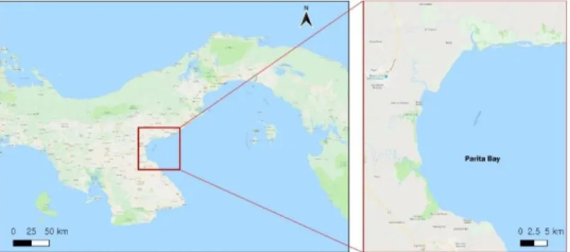
The site of this study is the Parita Bay located between latitude 8°18'40"N and longitude 80°13'37"W to latitude 7°57'18"N and longitude 80°21'49"W in the central Pacific side of Panama (Figure 1). The area belongs to the called ‘Dry Arc’ (the driest zone of the country) and is situated within Coclé, Herrera and Los Santos provinces. The study area comprises five (5) watersheds: Anton, Rio Grande, Santa Maria, Parita and La Villa rivers. Its extension is about 613 km2.
The zone is characterized by Dry Tropical and Dry Premontane Forests; and the annual precipitation can be <1000 mm, with the presence of tropical savanna weather (ANAM & UCCD, 2009). The mangroves species found in the region are: Laguncularia racemosa, Rhizophora mangle, Avicennia germinans,
Conocarpus erectus, acrostichum aureum, and Pelliciera rhizophorae. (ANAM
& ARAP, 2013).
There are two protected areas within the study zone:
a. Sarigua National Park. Established in 1984 with an extension of 47 km2,
although it is referred as of 80 km2 when including a great part of the sea
territory in Parita Bay. More than 50% of the protected area is concessioned to breeding-shrimp ponds for export. Additionally, it is located in an archaeological area of great importance for the study of cultural evolution in the Isthmus of Prehispanic Panama (CREHO-Ramsar, 2009).
b. Cenegon de Mangle Wildlife Refuge. Established in 1980 with an
approximated 9 km2 extension. It is located about 5 km from the community of
Paris in the district of Parita, in the estuary of the Santa Maria River. It borders the Sarigua National Park and possess one of the largest heron bird colonies known in Panama, as well as the largest colony of white ibis (Eudocimus albus) and large egret (Ardea alba) (CREHO-Ramsar, 2009).
6
Figure 1. Location of Study Area in Parita Bay, Panama. Source: google maps.
2. Data Selection and Image preprocessing
Five Landsat images (30 m spatial resolution) were downloaded from the United States Geological Survey’s (USGS) Earth Explorer website (https://earthexplorer.usgs.gov/) (Table 1). All images capture date belong to the ‘Dry’ season of the country which last from December to April (UNESCO, 2008). For the atmospheric and radiometric correction, the Surface reflectance products from USGS Landsat Ecosystem Disturbance Adaptive Processing System (LEDAPS) (USGS, 2018) and the Landsat surface reflectance code (LaSRC) (USGS, 2017) were used. The Landsat surface reflectance is processed calibrating raw DNs to TOA (Tops of atmosphere) reflectance and then corrected to surface reflectance using atmospheric parameters and DEM (Digital Elevation Model). These data are the most current high level and reliable products for atmospheric correction, readily available for ecologists (Young et al., 2017). However, as these are images from two different sensors, OLI and TM, it should be considered that the difference between them may lead to error in the analysis (Tuholske et al., 2017).
Each band image was clipped in order to extract the free-cloud study region for the analysis. However, for the 2009 period, due to cloud conditions, a composite of two images from December 2009 and January 2010 was created; though some clouds were present, which later were detected and extracted. Each clipped raster band image was used to construct a composite for the classification. The False Color combination of bands Near-Infrared (NIR), RED
7
and GREEN as RGB was used for mapping mangrove on the 1987, 1998 and 2019 images (Islam, Borgqvist, & Kumar, 2018; Jayanthi, Thirumurthy, Nagaraj, Muralidhar, & Ravichandran, 2018).; however, 2009-2010 images seemed to have better results for mapping mangrove on the SWIR, NIR, and RED combination (Gaw et al., 2018; Rahman, Tabassum, & Saba, 2017). Table 1. Data products used for the study
3. Image Classification
The false color composite for 1987, 1998, 2019 images were classified using a supervised classification with the Maximum Likelihood algorithm using the open free software QGIS 3.4 version (http://qgis.osgeo.org/) and the Semi-Automatic Classification plugin (Luca Congedo, 2016) (See Figure 2 for entire flow chart process). Maximum likelihood supervised classification has been widely used for mapping mangrove land cover (Heumann, 2011), and is considered as one of the most robust method for classifying mangroves based on traditional satellite remote-sensing data (Kuenzer, Bluemel, Gebhardt, Quoc, & Dech, 2011). The maximum likelihood classifier quantifies the variance and covariance of a spectral class pattern. It computes the statistical probability of a given pixel being a member of a specific land cover class assuming a normal distribution (Lillesand, Kiefer, & Chipman, 2015).
For the 2009-2010 composite image (SWIR, NIR, RED) it was used the Minimum distance algorithm Supervised classification, which specifically produced best results for that image. In this type of classification it is calculated
Satellite Sensor Product ID Date Path/r
ow Landsat 5 TM LT05_L1TP_012054_19870119_201702 15_01_T1 1987-01-19 12/54 Landsat 5 TM LT05_L1TP_012054_19980322_201612 26_01_T1 1998-03-22 12/54 Landsat 5 TM LT05_L1TP_012054_20091201_201610 17_01_T1 2009-12-01 12/54 Landsat 5 TM LT05_L1TP_012054_20100118_201610 17_01_T1 2010-01-18 12/54 Landsat 8 OLI LC08_L1TP_012054_20190127_201902 06_01_T1 2019-01-27 12/54
8
the mean, or average, spectral value in each band for each category and then a pixel of unknown identity may be classified by computing the distance between the value of the unknown pixel and each of the category mean (Lillesand et al., 2015). Additionally, it is not the first time for a land cover change analysis to use different algorithms-classified images (Rioja-Nieto et al., 2017).
Field survey (Feb-2019) Reference data (Google Earth, Orthophotos) Output: Error Confusion Matrix
Time Change Detection
NDVI Time series analysis
Land cover time change analysis
Output: NDVI Change matrix. NDVI Change
map
Output: Land Use-Cover Change
matrix
Analysis of Environmental Variables
Temperature (Min, Max, Mean), Rainfall Analysis of Change within Protected areas vs.
Non-protected areas
Finding possible drivers of change
NDVI trend of Change in Mangrove and Other
vegetation classes. (Boxplots)
Data Collection (Landsat 5 TM, Landsat 8 OLI) NDVI reclassification Output: Density Map Classification of Land Cover/ Land Uses
Training areas definition Supervised Classification (Maximum likelihood, Minimum distance) Output: land cover map Post-processing
-Masking all pixels over 35 m asl with a DEM mask & -Removing Isolated Pixels
Density Analysis
Pre-processing
(Radiometric correction, Cloud detection and masking
Accuracy assessment of land cover classification
NDVI, Composite stacking combinations.
(RGB; NIR-RED-GREEN; SWIR1, NIR, RED)
9
For each satellite imagery, it was defined a new set of training areas. To define training areas the analyst must have a certain knowledge about the study site, different form an unsupervised classification (Wulder & Franklin, 2003). In this case, the Land Use-Cover Map from the Ministry of Environment of Panama (from 2012) was used as a reference for the definition of training areas and classification. This map is legally approved and recognized by the Panamanian government through the Resolution N° DM-0067-2017 since February 16th,
2017. It was built-up using ‘Rapideye’ satellite images with 5m resolution and field surveys. For the purpose of this study, five (5) Land Use-Cover classes were defined: 1) Mangrove; 2) Water (Rivers, ponds, Sea); 3) Aquaculture ponds and Salt Pans (AS); 4) Other vegetation (Grassland, Shrubs, Crops, Upland forest, marshes); 5) Others (Bare Soil & Built-up). Furthermore, as the spectral signature from the Aquaculture and Saltpan class can be mixed and confused with the water and bare soil class, it resulted more convenient to perform a visual classification of the Aquaculture pond and Saltpans category. This method has been used in many studies, such as (Alatorre et al., 2015; Jayanthi, Thirumurthy, Muralidhar, & Ravichandran, 2018; Thomas et al., 2017).
After classification, it was necessary to perform image post processing for removing of isolated pixels. First, all mangrove pixels located at high elevations were masked using the Digital Elevation Model Shuttle Radar Topography Mission (SRTM). An SRTM image (1-arc resolution) was used to make a mask for elevations over 35m asl, because Mangrove in Panama have been reported to grow until 30 m height (ANAM & ARAP, 2013) and mangrove are found in intertidal areas not higher than 5 m asl (Gaw et al., 2018). For other post processing, the option ‘Edit Raster’ and ‘Raster dilation’ from the semi-automatic classification plugin (Luca Congedo, 2016) was used.
10
4. Field Ground Truth and Accuracy Assessment
We performed a field survey from February 8th to 12th 2019 for the accuracy
assessment of 2019 image. The reference data must be independent from the data being tested to ensure objectivity of the assessment (Congalton & Green, 2009). For that reason, the field data obtained from the ground truth was not used in the setting of training areas for the supervised classification and was strictly kept for the accuracy assessment. Thirteen places were visited including: ‘La Camaronera’, ‘El Coco’, ‘Puerto Posada’, ‘El Gago’, ‘Aguadulce’ port, ‘El Gallo’, ‘El Salado’, ‘Boca de Parita’, ‘El Reten’ beach, ‘El Agallito’ beach, ‘Monagre’ beach, and the protected areas ‘Sarigua’ National Park and ‘Cenegon de Mangle’ Wildlife Refuge.
The methodology for the sampling was a stratified random sampling limited to realistic distance from the roads or access ways (Congalton & Green, 2009) because some areas had restricted access or are deep dense mangrove zones, turning dangerous for the team. Using a Garmin ‘GPSMAP 64S’ we took 330 ground control points (GCP). Afterward, it was built a new set of 125 points inside homogenous class regions nearest to the original GCP, then buffered into a 45 m radius to make sure that the area size is bigger than the small spatial resolution of a Landsat pixel (30m). Additionally, another set of 125 random sampling points was created to complement the previous GCPs from the field, making 250 validation points in total. These points, were later verified using google earth imagery to validate the accuracy of the entire image (Tilahun, 2015). A pixel-based error matrix and Kappa coefficient were calculated. A similar process with 250 random sample points was performed also for the 2009-2010 image and validated through google earth imagery and orthophotography from the year 2009 provided by the Ministry of Environment. Images from 1987 and 1998 were not validated due to lack of data.
11
5. NDVI Analysis
In addition to the land use-cover classification, a Normalized Difference Vegetation Index (NDVI) reclassification was also performed as mangrove cover extent only provides information about area change (quantity). To know about the quality change (greenness), NDVI time series map is a good resource (Alatorre et al., 2015). The NDVI is the most widely used and robust index for vegetation analysis (Kuenzer et al., 2011; Wulder & Franklin, 2003). This index provides information about the photosynthetic capacity of absorption of plants and leaf resistance to water vapor transfer (Ruimy, Saugier, & Dedieu, 1994). Also NDVI is related with canopy closure, leaf area index (Green, Mumby, Edwards, Clarck, & Ellis, 1993; Kovacs, Wang, & Flores-Verdugo, 2005), aboveground biomass, and net primary productivity (Castillo, Apan, Maraseni, & Salmo, 2017; Yengoh, Dent, Olsson, Tengberg, & Compton, 2015). Its relationship with the photosynthetically active radiation and greenness makes it a good indicator for vegetation health (Servino et al., 2018). The NDVI values range from -1 to 1. Normally for vegetation it ranges from 0.1 to 0.7, the high values indicate a high vegetation activity, therefore a good vegetation health, while low values indicate stressed or unhealthy vegetation (Flores-Cárdenas et al., 2018). NDVI was calculated for each satellite image with the following equation (Rouse et al., 1973):
𝑁𝐷𝑉𝐼 =
𝑁𝐼𝑅−𝑅𝐸𝐷𝑁𝐼𝑅+𝑅𝐸𝐷 (1)Where NIR is the near infrared band (5 for OLI and 4 for TM sensors) and RED is the red band (4 for OLI, and 3 for TM sensors). The next step was to reclassify the NDVI to identify the vegetation density based on the range of values given in 2019 image, which ranged from -0.63 to 0.92 (Ehsan & Kazem, 2016; El-Gammal, Ali, & Samra, 2013; Tran & Fischer, 2017; Zaitunah, Samsuri, Ahmad, & Safitri, 2018). NDVI was categorized as follow: NDVI ≤0, (Water or aquaculture); 0<NDVI≤0.23, as Low density (Bare soil to grassland);
12
0.23<NDVI≤0.46, as Medium density; 0.46<NDVI≤0.69, as High density; and NDVI>0.69, as Very high density.
This information is applicable for the NDVI of all classes in the study area and may include some bias mainly due to crop cover, between harvested and non-harvested fields. However, to know the changes in NDVI of the mangrove cover specifically, it was performed a random sampling of 500 points in the ‘mangrove’ layer with NDVI values (Figure 3). Finally, these points were displayed in boxplots, to know the trend of change of NDVI in Mangrove class. Same procedure was performed for ‘Other vegetation’ cover in Parita Bay. .
Figure 3. Random sampling of 500 pixel points of NDVI values in unchanged mangrove cover.
6. Land Cover-Use Change (LUCC) detection
Change Detection for the classified Land Use-Cover images and the other reclassified NDVI maps was developed by using the Semi-Automatic plugin
13
(Luca Congedo, 2016) and MOLUSCE (Modules of Land Use Change Evaluation) plugin (Rahman et al., 2017) in QGIS 3.4 and 2.18.
7. Analysis in Protected Areas
Additionally, a Land Use-Cover Change detection for Protected and Unprotected areas was performed (Figure 4). All classified images, were masked with the Protected Areas ‘Cenegon de Mangle Wildlife Refuge’ and ‘Sarigua National Park’ shapefiles provided by the Ministry of Environment of Panama.
Figure 4. Protected Areas located in the study region of Parita Bay. a) Study region Landsat 8 RGB composite raster. b) ‘Cenegon de Mangle’ Wildlife Refuge and ‘Sarigua’ National Park zoomed area.
8. Analysis of Environmental variables in the study area
To investigate the possible drivers of change of the mangrove cover in Parita Bay some climatic variables were analyzed. Rainfall, Mean, Maximum and
14
Minimum Temperature data were obtained from meteorological stations on the site, downloaded from ETESA (http://www.hidromet.com.pa/open_data.php) for the year 1986 to 2018.
Rainfall data was obtained from four (4) meteorological stations within Parita Bay: ‘Parita’, ‘Los Santos’, ‘Puerto Posada’ and ‘Rio Hondo’, located in Herrera, Los Santos, and Cocle provinces (Figure 5). The One-way ANOVA test was used to compare statistically each meteorological station. Temperature data was only available in ‘Parita’ and ‘Los Santos’ stations. Annual accumulative rainfall and average temperature was calculated in order to see its behavior in time. Additionally, based on (Galeano, Urrego, Botero, & Bernal, 2017) the accumulative rainfall and average temperature 3 months (90 days) before the date of satellite image capture were estimated in order to have a comprehensive overview of the scenario behind each Landsat image. As there are not meteorological stations inside the protected areas, the closer stations, in this case ‘Parita’ and ‘Los Santos’ were considered as to correspond to the protected area reference rainfall data. This is based in the document of the first communication about climate change to the IPCC in the year 2000 (ANAM, 2000), in which the Panamanian government used the data from ‘Los Santos’ station to analyze the Sarigua National Park environmental status. Some of the graphics for this study were performed using R program (R Core Team, 2013) and SigmaPlot Version 12.5.
15
Figure 5 View of the Meteorological stations in Parita Bay. Rainfall data was obtained from ‘Rio Hondo’, ‘Puerto Posada’, ‘Parita’ and ‘Los Santos’ stations. Temperature data was obtained from ‘Parita’ and ‘Los Santos’ stations. ‘Enrique Ensenat’ and ‘La Estrella’ do not provide complete data and
were discontinued years ago.
(source:http://www.hidromet.com.pa/open_data.php). Rio Hondo P.Posada Parita Los Santos Enrique Ensenat La Estrella
16
III. Results
1. Classification Accuracy
The overall accuracy for the 2019 classified images is 87% with a Kappa coefficient 0.83 which is considered a good level of agreement between classifiers (Wulder & Franklin, 2003) (Table 2). Classification for the 2009-2010 image also shows a strong agreement between the reference and classified data as Overall Accuracy is 90% and Kappa coefficient 0.86 (Table 3). In general, it can be said that most errors in the mangrove cover classification fall upon the Producer (error of omission) rather than the User (errors of commission); in other words, mangrove class tends to be underestimated in the map. For example, one source of error we found on field is that some mangroves have a small size and are regenerating in the middle of a very dry bare soil near ‘Sarigua’ and ‘Cenegon de Mangle’ Protected Areas. Therefore, in the map, it is classified as bare soil class, but in the field, it seems as mangroves regenerating, consequently, it is identified as mangrove class, generating errors of omission. For both images ‘Bare soil & Built-up’ class (No.5) tends to have the lowest accuracy, mainly due to the crops, which appear like bare soil class in the classifier because have been harvested, while in the reference may appear as crops. However, ‘Bare soil & Built-up’ is not a category of concern for this study as this analysis is more focus in Mangrove and Aquaculture & Salt-Pan (AS) classes.
17
Table 2. Pixel-based Error Matrix for the classified 2019 Landsat Image. AS= Aquaculture and Saltpans, OV= Other vegetation, BB=Bare soil & Built-up
Pixel-based Error Matrix for 2019 Landsat Image Classification
Map classifier
Reference classifier User's accuracy Producer's Accuracy M W AS OV BB Total Mangrove 483 0 0 0 0 483 100.00 75.82 Water 0 58 0 0 0 58 100.00 98.31 AS 21 0 298 0 7 326 91.41 100.00 Other vegetation 105 1 0 528 26 660 80.00 96.00 BB 28 0 0 22 158 208 75.96 82.72 Total 637 59 298 550 191 1735 Overall Accuracy 87.9 Kappa hat classification 0.83
Table 3. Pixel-based Error Matrix for the classified 2009-2010 composite Landsat Image. M= mangrove, W= water, AS= Aquaculture and Saltpans, OV= Other vegetation, BB=Bare soil & Built-up
Pixel-based Error Matrix for 2009-2010 Lansdat Image Classification
Map classifier Reference classifier User's accuracy Producer's Accuracy M W AS OV BB Total Mangrove 374 0 3 0 2 379 98.68 83.86 Water 0 97 0 0 0 97 100.00 100.00 AS 0 0 352 10 0 362 97.23757 99.15 Other vegetation 66 0 0 641 38 745 86.04 91.31 BB 6 0 0 51 127 184 69.02 76.05 Total 446 97 355 702 167 1767 Overall Accuracy 90.0 Kappa hat classification 0.86
18
2. Land Use-Cover Change (LUCC) Detection and
mangrove estimation in Parita Bay
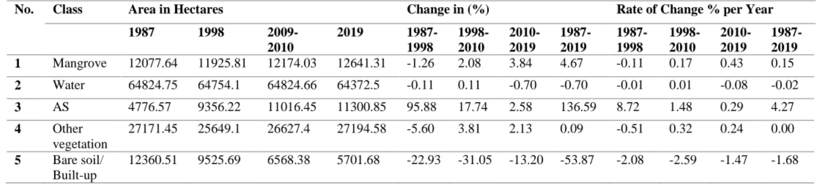
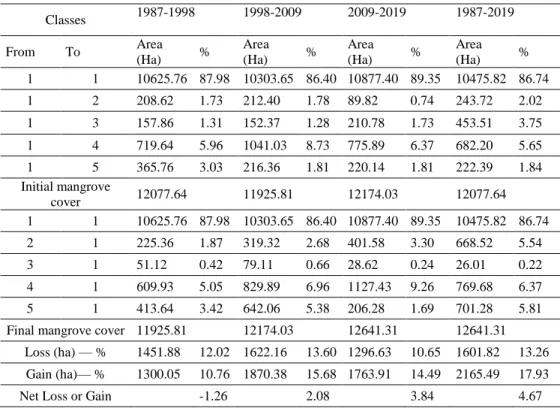
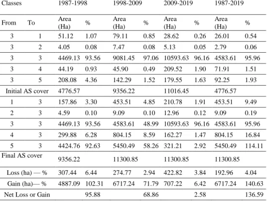
Land Use-Cover classified maps are shown in Figure 6. Over the 32-year analysis, mangroves had increased in extent more than 500 hectares (4.7%), with an annual average rate of change of 0.15%. However, during the period from 1987 to 1998 there is an evident decrease in mangrove cover (151.83 ha) with a rate of -0.11% (Table 4). In spite of this decrease, eventually mangroves developed an increment through the next two decades. From 1998 to 2010, mangrove area experienced a rise (248.22 ha) with an annual rate of 0.17%; to finally end in 2019 with an increase rate of 0.43% per year, meaning a growth of 467.28 ha. The ‘Other Vegetation’ class, mainly composed of grasslands, shrubs, crops, marshes and some upland forest, also faced a decline in extent from 1987 to 1998, and similar to mangrove cover, raised up in the next 20 years until 2019. Throughout this time, it is also observed a great expansion of (AS) activities (4579.65 ha) growing at an annual rate of 8.72% continuing to increase for the next two decades, but in a lower rate of 1.48% and 0.29% respectively. The graphic at (Figure 7) presents Land cover extent change of ‘Mangrove’, ‘Aquaculture & Salt-Pan’ (AS), ‘Other vegetation’ and ‘Bare soil & Built-up’ (BB) classes, ‘Water’ class was excluded, as it represents a greater area on the map causing that changes in other classes would not be noticed; plus, its changes are negligible. Additionally, a closer look to the mangrove cover change is shown in Figure 8. Results from the mangrove cover matrix of change indicates that through the 32 years 86.7% of the mangroves extent remained the same and 13.26% were lost, mostly due to ‘Other vegetation’ and ‘Aquaculture-Saltpan’ activities (Table 5). Nevertheless, mangroves gain in the site come from the ‘Water’ class (5.54%), ‘Other vegetation’ (6.37%), and ‘Bare Soil’ (5.81%). On the other side, (AS) activities have increased 136.6% through the 32 years, and according to the aquaculture and saltpans (AS) matrix of change, this expansion is predominantly due to bare soil (BB) conversion, representing a 114.1% (5450.49 ha); while mangrove conversion contribute to 9.5% of AS increase, about 453.5 ha (Table 6).
19
Table 4. Land Use-Cover area change and rate of change in Parita Bay from 1987 to 2019. The composite image from 2009-2010, for practical reasons is defined as only 2010 for the Change Analysis.
No. Class Area in Hectares Change in (%) Rate of Change % per Year
1987 1998 2009-2010 2019 1987-1998 1998-2010 2010-2019 1987-2019 1987-1998 1998-2010 2010-2019 1987-2019 1 Mangrove 12077.64 11925.81 12174.03 12641.31 -1.26 2.08 3.84 4.67 -0.11 0.17 0.43 0.15 2 Water 64824.75 64754.1 64824.66 64372.5 -0.11 0.11 -0.70 -0.70 -0.01 0.01 -0.08 -0.02 3 AS 4776.57 9356.22 11016.45 11300.85 95.88 17.74 2.58 136.59 8.72 1.48 0.29 4.27 4 Other vegetation 27171.45 25649.1 26627.4 27194.58 -5.60 3.81 2.13 0.09 -0.51 0.32 0.24 0.00 5 Bare soil/ Built-up 12360.51 9525.69 6568.38 5701.68 -22.93 -31.05 -13.20 -53.87 -2.08 -2.59 -1.47 -1.68
20
Table 5. Matrix of Change for Mangrove Class from 1987 to 2019. Class 1=Mangrove, 2=Water, 3=Aquaculture and Salt-Pans, 4=Other vegetation, and 5=Bare soil and Built-up.
Classes 1987-1998 1998-2009 2009-2019 1987-2019 From To Area (Ha) % Area (Ha) % Area (Ha) % Area (Ha) % 1 1 10625.76 87.98 10303.65 86.40 10877.40 89.35 10475.82 86.74 1 2 208.62 1.73 212.40 1.78 89.82 0.74 243.72 2.02 1 3 157.86 1.31 152.37 1.28 210.78 1.73 453.51 3.75 1 4 719.64 5.96 1041.03 8.73 775.89 6.37 682.20 5.65 1 5 365.76 3.03 216.36 1.81 220.14 1.81 222.39 1.84 Initial mangrove cover 12077.64 11925.81 12174.03 12077.64 1 1 10625.76 87.98 10303.65 86.40 10877.40 89.35 10475.82 86.74 2 1 225.36 1.87 319.32 2.68 401.58 3.30 668.52 5.54 3 1 51.12 0.42 79.11 0.66 28.62 0.24 26.01 0.22 4 1 609.93 5.05 829.89 6.96 1127.43 9.26 769.68 6.37 5 1 413.64 3.42 642.06 5.38 206.28 1.69 701.28 5.81 Final mangrove cover 11925.81 12174.03 12641.31 12641.31
Loss (ha) — % 1451.88 12.02 1622.16 13.60 1296.63 10.65 1601.82 13.26 Gain (ha)— % 1300.05 10.76 1870.38 15.68 1763.91 14.49 2165.49 17.93 Net Loss or Gain -1.26 2.08 3.84 4.67
21
Table 6 Matrix of Change for AS Class from 1987 to 2019. Class 1=Mangrove, 2=Water, 3=Aquaculture and Saltpans, 4=Other vegetation, and 5=Bare soil and Built-up. Classes 1987-1998 1998-2009 2009-2019 1987-2019 From To Area (Ha) % Area (Ha) % Area (Ha) % Area (Ha) % 3 1 51.12 1.07 79.11 0.85 28.62 0.26 26.01 0.54 3 2 4.05 0.08 7.47 0.08 5.13 0.05 2.79 0.06 3 3 4469.13 93.56 9081.45 97.06 10593.63 96.16 4583.61 95.96 3 4 44.19 0.93 45.90 0.49 209.52 1.90 71.91 1.51 3 5 208.08 4.36 142.29 1.52 179.55 1.63 92.25 1.93 Initial AS cover 4776.57 9356.22 11016.45 4776.57 1 3 157.86 3.30 453.51 4.85 210.78 1.91 453.51 9.49 2 3 4.59 0.10 9.09 0.10 12.96 0.12 9.09 0.19 3 3 4469.13 93.56 4583.61 48.99 10593.63 96.16 4583.61 95.96 4 3 299.88 6.28 804.15 8.59 162.27 1.47 804.15 16.84 5 3 4424.76 92.63 5450.49 58.26 321.21 2.92 5450.49 114.11 Final AS cover 9356.22 11300.85 11300.85 11300.85 Loss (ha) — % 307.44 6.44 274.77 2.94 422.82 3.84 192.96 4.04 Gain (ha)— % 4887.09 102.31 6717.24 71.79 707.22 6.42 6717.24 140.63 Net Loss or Gain 95.88 68.86 2.58 136.59
22
Figure 6. Parita Bay Land Use-Cover classification of the images from 1987, 1998, 2009-2010 and 2019. Classes in the graphic are: Mangrove, Water, Aquaculture & Saltpans (AS), Other vegetation and Bare Soil & Built-up (BB).
Figure 7. Graphic of Land Cover- Land Use Change in Parita Bay for Mangrove, Aquaculture & Salt-Pans (AS), Other vegetation and Bare soil & Built-up (BB) classes. Water category was excluded.
23
Figure 8. Mangrove cover extent (in hectares) in Parita Bay for the years 1987, 1998, 2009-2010 and 2019.
3. NDVI Classes Changes on time
Similar to the Land Use-Cover change detection, NDVI classes’ time series analysis was also developed (Table 7 and Figure 9). This will help us to understand the changes of NDVI along the entire study area. One thing to consider is that this information may include some bias mainly due to crop cover, between harvested and non-harvested crops. Results from the NDVI density class changes shows that ‘High’ (0.46<NDVI≤0.69) and ‘Very High’ (>0.69) density classes experienced a decreased from 1987 to 1998, followed by an increase from 1998 to 2009-2010 to finally experience another moderate decline until 2019. However, ‘Very High’ NDVI class stayed higher than what it was in the year 1987. The image from 1998 contain the largest amount of ‘Medium’(0.23<NDVI≤0.46) density and keeps a high cover of ‘Low’ density class (0<NDVI≤0.23), which is composed mainly of bare soil or spare grassland and shrubs. In fact, it is noticeable that 1998 image looks less greener compared with the others (Figure 10), this because it has the lowest amount of ‘High’ and ‘Very High’ density cover.
24 Table 7. NDVI Density Classes Change between 1987 and 2019
Range Class Area in Hectares Change in % Annual rate of Change
1987 1998 2009-2010 2019 1987-1998 1998-2009 2009-2019 1987-2019 1987-1998 1998-2010 2010-2019 1987-2019 NDVI ≤0 No Vegetation 63260.19 66435.84 61098.75 64704.06 5.02 -7.90 5.90 2.42 0.46 -0.66 0.66 0.08 0< NDVI≤0.23 Low density 13775.94 14648.22 13474.26 11105.28 6.33 -7.98 -17.58 -19.32 0.58 -0.66 -1.95 -0.60 0.23<NDVI≤0.46 Medium density 18905.94 25050.15 5920.47 15387.75 32.50 -76.35 159.91 -18.53 2.95 -6.36 17.77 -0.58 0.46<NDVI≤0.69 High density 17649.81 10436.13 16644.6 15830.64 -40.87 59.59 -4.89 -10.25 -3.72 4.97 -0.54 -0.32
NDVI>0.69 Very high
density
7619.04 4640.58 23927.76 14038.11 -39.09
25
Figure 9. NDVI Density classes area (ha) changes in the Parita Bay from 1987 to 2019. No vegetation level (NDVI≤0) was excluded, as it represents water cover, which has great extension on the map, producing no visible changes for other classes.
Figure 10. Parita Bay NDVI density map for a) 1987, b)1998, c)2009-2010, and d) 2019. No vegetation (NDVI≤0), Low vegetation (0<NDVI≤0.23), Medium (0.23<NDVI≤0.46), High (0.46<NDVI≤0.69), Very High (NDVI>0.69).
Low density Medium density High density Very high density
A rea (ha) 0 10000 20000 30000 1987 1998 2009-2010 2019
26
4. NDVI trend in mangrove and other vegetation
covers
The sampled NDVI values for the mangrove cover present a skewed left distribution, notice on the boxplots (Figure 11), which tells us that mangroves on the site present high or very high NDVI values (close to 1). Mangroves in Parita Bay present a mean NDVI increase in the 32 years, starting with a decline during the 1987-1998 period (from 0.70 to 0.67), followed by an increase on the 2009-2010 cover (0.81), to finish with a slight increase on 2019 image (0.82), this trend coincides with the mangrove land cover change analysis (Figure 12).
Figure 11. Boxplots of Mangrove NDVI samples from 1987 to 2019. Represents the 500 random sampling on the NDVI raster for mangrove cover only, for the four (4) points of time.
27
Figure 12. Mangrove area change and NDVI trend for each satellite image in Parita Bay.
When the same analysis is performed for the category No.4 (Other vegetation), distributions are irregular (Figure 13), principally because this category is composed of many types of vegetation, which comprises widest range in NDVI from that of mangrove class. For ‘Other vegetation’ class, the NDVI mean of 1987 was 0.46, while the year 1998 presented the lowest NDVI (0.35, 0.32 and 0.30), and the distribution is skewed right. Eventually, in 2009-2010 NDVI rises the highest (0.71), and the distribution is skewed left. These results explain why the NDVI density map shows a greener appearance with an increase in ‘High’ and ‘Very high’ NDVI categories for that year. Meaning that the decrease in ‘High’ and ‘Very High’ density class of the year is due to crops, grassland, shrubs and upland forest, rather than by the mangrove cover itself. In spite of this, is evident that both ‘Mangrove’ and ‘Other vegetation’ experienced a decline in the year 1998 and then lift up on the 2009-2010 period.
28
Figure 13. Boxplots of Other vegetation NDVI values sampled from 1987 to 2019. Represents the 500 random sampling on the Class No.4 (Other vegetation) only, for the four (4) points of time.
5. Mangroves changes in Protected vs. Unprotected Area
A Land Use - Cover Change Analysis was completed for each protected area and for the unprotected part to compare differences in the rate of change (Figure 14). Mangrove changes inside the protected areas present different trend comparing with the previous overall analysis. The graph in Figure 15 presents the difference in the rate of change between the Unprotected and Protected Areas. Mangrove Cover declined during the first period (1987 to 1998), and this decrease presents a higher rate in Protected areas than in Unprotected regions (-0.17% vs -0.11%); later on, it increased during the 1998-2010 period (0.56%), but far ahead decreased (-0.11%) from 2010 to 2019; while mangroves in unprotected areas have increased 0.12% and 0.50%, respectively. On another point, in Sarigua, the only protected area containing aquaculture activity (AS), there was an increase of 187.7% for the period of 1987 to 1998, and 245.1% in total from 1987 to 2019. These values doubled those of the unprotected regions of 85% and 123.7% for the same periods respectively (Tables 8 and 9). Matrix of change in mangrove cover for each protected area reveal that the major class producing mangrove losses and gains is ‘Other vegetation’ (Tables 10 and 11).
29
Figure 14 Cenegon de Mangle Wildlife Refuge and Sarigua National Park extracted Land Use-Cover maps from 1987, 1998, 2009-2010, and 2019 in Parita Bay.
Figure 15. Comparison of the annual rate of change for both Protected versus Unprotected areas. Accumulative results from 1987 to 2019 are shown in the last two bars on the graph.
Period 1987-1998 1998-2010 2010-2019 1987-2019 Rate of Chan g e per y ear ( %) -0.4 -0.2 0.0 0.2 0.4 0.6 0.8 Mangrove protected Mangrove unprotected
30
Table 8. Land Use-Cover loss and gains in Cenegon de Mangle Wildlife Refuge and Sarigua National Park
No. Class Total for both protected area in hectares
Change in % Rate of Change % per Year
1987 1998 2009 2019 1987-1998 1998-2009 2009-2019 1987-2019 1987-1998 1998-2009 2009-2019 1987-2019 1 Mangrove 1459.71 1432.89 1528.83 1514.07 -1.84 6.70 -0.97 3.72 -0.17 0.56 -0.11 0.12 2 Water 1291.77 1288.08 1278.81 1238.85 -0.29 -0.72 -3.12 -4.10 -0.03 -0.06 -0.35 -0.13 3 AS 506.79 1457.91 1812.33 1748.79 187.68 24.31 -3.51 245.07 17.06 2.03 -0.39 7.66 4 Other vegetation 316.8 388.17 523.89 579.06 22.53 34.96 10.53 82.78 2.05 2.91 1.17 2.59 5 Bare soil/ Built-up 1939.32 947.34 370.53 433.62 -51.15 -60.89 17.03 -77.64 -4.65 -5.07 1.89 -2.43
Table 9. Land Use-Cover loss and gains in the unprotected region of the study area
No. Class Area in hectares Change in % Rate of Change % per Year
1987 1998 2009 2019 1987-1998 1998-2010 2010-2019 1987-2019 1987-1998 1998-2010 2010-2019 1987-2019 1 Mangrove 10617.66 10492.65 10645.02 11126.97 -1.2 1.5 4.5 4.8 -0.11 0.12 0.50 0.15 2 Water 63532.62 63465.66 63545.4 63133.29 -0.1 0.1 -0.6 -0.6 -0.01 0.01 -0.07 -0.02 3 AS 4269.78 7898.31 9204.12 9552.06 85.0 16.5 3.8 123.7 7.73 1.38 0.42 3.87 4 Other vegetation 26854.65 25260.93 26103.51 26615.52 -5.9 3.3 2.0 -0.9 -0.54 0.28 0.22 -0.03 5 Bare soil/ Built-up 10421.19 8578.35 6197.85 5268.06 -17.7 -27.8 -15.0 -49.4 -1.61 -2.31 -1.67 -1.55
31
Table 10. Matrix of Change for Mangrove Class in Cenegon de Mangle from 1987 to 2019. Class 1=Mangrove, 2=Water, 4=Other vegetation, and 5=Bare soil and Built-up.
Classes 1987-1998 1998-2009 2009-2019 1987-2019 From To Area (Ha) % Area (Ha) % Area (Ha) % Area
(Ha) % 1 1 582.30 91.27 594.36 96.11 632.61 93.40 604.35 94.72 1 2 1.35 0.21 7.65 1.24 1.35 0.20 4.41 0.69 1 3 47.25 7.41 16.20 2.62 41.22 6.09 27.54 4.32 1 4 7.11 1.11 0.18 0.03 2.16 0.32 1.71 0.27 Initial mangrove cover 638.01 618.39 677.34 638.01 1 1 582.30 91.27 594.36 96.11 632.61 93.40 604.35 94.72 2 1 1.26 0.20 0.45 0.07 7.47 1.10 2.97 0.47 3 1 24.93 3.91 62.82 10.16 30.69 4.53 44.28 6.94 4 1 9.90 1.55 19.71 3.19 0.18 0.03 19.35 3.03 Final mangrove cover 618.39 677.34 670.95 670.95 Loss (ha) — % 55.71 8.73 24.03 3.89 44.73 6.60 33.66 5.28 Gain (ha)— % 36.09 5.66 82.98 13.42 38.34 5.66 66.60 10.44 Net Loss or Gain -3.08 9.53 -0.94 5.16
32
Table 11. Matrix of Change for Mangrove Class in Sarigua National Park from 1987 to 2019. Class 1=Mangrove, 2=Water, 3=Aquaculture and Saltpans, 4=Other vegetation, and 5=Bare soil and Built-up.
Classes 1987-1998 1998-2009 2009-2019 1987-2019 From To Area (Ha) % Area (Ha) % Area (Ha) %
Area (Ha) % 1 1 745.92 90.78 753.21 92.48 786.33 88.75 721.44 87.80 1 2 11.34 1.38 3.87 0.48 9.27 1.05 10.62 1.29 1 3 9.18 1.12 15.3 1.88 7.92 0.89 19.53 2.38 1 4 27.27 3.32 36.72 4.51 68.04 7.68 50.31 6.12 1 5 27.99 3.41 5.40 0.66 14.40 1.63 19.80 2.41 Initial mangrove cover 821.70 814.50 885.96 821.70 1 1 745.92 90.78 753.21 92.48 786.33 88.75 721.44 87.80 2 1 13.86 1.69 42.39 5.20 21.78 2.46 60.03 7.31 3 1 7.92 0.96 5.31 0.65 2.34 0.26 4.32 0.53 4 1 29.34 3.57 25.29 3.10 28.08 3.17 28.62 3.48 5 1 17.46 2.12 59.76 7.34 4.59 0.52 28.71 3.49 Final mangrove cover 814.50 885.96 843.12 843.12 Loss (ha) — % 75.78 9.22 61.29 7.52 99.63 11.25 100.26 12.20 Gain (ha)— % 68.58 8.35 132.75 16.30 56.79 6.41 121.68 14.81 Net Loss or Gain -0.88 8.77 -4.84 2.61
33
6. Local Climatic Variables Analysis
6.1 Rainfall
The One-way ANOVA test between stations show there is not significant difference between Parita and Los Santos station (p= 0.5) and between ‘Puerto Posada’ and ‘Rio Hondo’ stations (p=0.6), but there is a significant difference between Parita and Puerto Posada, Rio Hondo and Los Santos, Parita and Rio Hondo, Los Santos and Puerto Posada (p< 0.01) (Appendix C). This makes sense as Parita and Los Santos are closer to each other, while Puerto Posada and Rio Hondo are also closer between them but far from the other two. The mean annual accumulative rainfall in Puerto Posada and Rio Hondo stand higher than in the Parita and Los Santos stations over the 32 years (Figure 16). Rainfall register (3) three months (90 days) before each capture initially start with 185~377 mm during 1987 image; next period (1998) experienced a decreased in precipitation with only 7.5 mm in Parita station, 1.8 mm in Los Santos and 0 mm in P. Posada and Rio Hondo (Table 12); In contrast, 2009 image present the higher rainfall register of 424~532 mm. However, data for the 2019 image was only available in Parita station with a register of 189.5 mm (Figure 17).
Figure 16. Annual accumulative rainfall in Parita Bay from January 1986 to December 2018. Each point represents the average accumulative daily
Year 1980 1985 1990 1995 2000 2005 2010 2015 2020 R ainf all (mm ) 0 500 1000 1500 2000 2500 3000 Parita Los Santos Puerto Posada Rio Hondo Linear regression
34
rainfall calculated for each year from Parita, Los Santos, Puerto Posada, and Rio Hondo stations.
Figure 17. Rainfall 3 months before the date of capture of each Landsat imagery. Each bar represents the accumulative mean rainfall calculated 90 days before the capture.
Table 12. Accumulative Rainfall (mm) 90 days before each capture
Date of capture Closer to Protected Areas Unprotected Areas
Parita Los Santos Puerto
Posada Rio Hondo 19-Jan-87 377.9 185.2 259.6 234.7 22-Mar-98 7.5 1.8 0 0 01-Dec-09 532.7 424.3 512.8 529 *27/01/2019 189.5 0 0 1.1
*Lack of data for this period. Information available only for Parita Station.
6.2 Temperature
Same as rainfall data, Average Annual Maximum, Mean and Minimum local Temperature was calculated (Figure 18). The 32-year period analysis for Parita Bay shows Maximum Temperature ranges between 31 and 34°C, Mean Temperature between 27 and 29 °C, and Minimum Temperatures between 22 to 24 °C. The Maximum Temperature (3) Three months before the image capture date are 31.4, 33.7, 32.1, and 31.9 °C for 1987, 1998, 2009-2010, and 2019 images, respectively. In the same order, Mean
Dates of capture *19/01/1987 *22/03/1998 *01/12/2009 *27/01/2019 R ainf all (mm ) 0 100 200 300 400 500 600 Parita Los Santos Puerto Posada Rio Hondo
35
Temperature are 27.2, 29.1, 28.0, and 27.5 °C, while Minimum Temperature are 23, 24.6, 24, and 23.1 °C.
Figure 18. Minimum, Mean and Maximum Temperature in Parita Bay from 1986 to 2019. From top to bottom (left side): Maximum annual Temperature; Mean annual Temperature; Minimum annual Temperature; From top to bottom (right side): Maximum Temperature in Parita Bay 3 months before the capture date of Landsat Images; Mean Temperature in Parita Bay 3 months before the capture date of Landsat images; Minimum Temperature in Parita Bay 3 months before the capture date of Landsat images.
36
IV. Discussion
While generally other studies have reported a mangrove net loss in their Time-Series Analysis (Brown, Pearce, Leon, Sidle, & Wilson, 2018; Gaw, Linkie, & Friess, 2018; Mondal, Trzaska, & De Sherbinin, 2018; Polidoro et al., 2010; Tuholske, Tane, López-Carr, Roberts, & Cassels, 2017), this study reports an overall increase in mangrove area. (Hamilton & Casey, 2016) conveyed that global annual mangrove deforestation rate was reaching up to 0.39% since the year 2000; however, our analysis for the last decade (2010-2019) in Parita Bay, reflects a 0.43% annual rate increasing trend. From 1987 to 2019, mangrove area increased in total 4.67%. However, our study is not the only one claiming a mangrove expansion, some other land cover change studies have reported an increase of mangrove forest area as well (Godoy, De Andrade Meireles, & De Lacerda, 2018; Hsu & Lee, 2018; Son, Thanh, & Da, 2016). For example, (Bianchi et al., 2013) found that mangroves have replace marshes over the past 60 years, in the Golf of Mexico. In addition (Wang, Cao, Guan, Wu, & Wang, 2018) registered an increase in mangrove cover at a rate of 5.5% from 1995 to 2014 in Fujian, China.
In Parita Bay, 86.7% of the mangrove area remained same, and 13.26% was lost due to mainly ‘Other vegetation’ and ‘Aquaculture-Saltpan’ activities during the 32 years. These results are in line with the known fact that agriculture, aquaculture and saltpans are the main anthropogenic drivers of global mangrove forest loss (Thomas et al., 2017). At the same time, mangrove cover expanded in a 17.93%, principally from ‘Water’, ‘Other vegetation’ and ‘Bare Soil’ classes conversion, meaning natural regeneration (seaward expansion) and restoration programs have great influenced on that increase. If we observe in detail, during 1987 to 1998 period, the net loss in mangrove area (1.26%) was also accompanied with a greenness decline (‘High’ and ‘Very High’ NDVI decreased 40.9% and
37
39.1% respectively). This decline in NDVI also coincides with a drought period and an increase in temperature 90 days before the capture of the image. Not uncommon, NDVI has been related with precipitation regimes, for example, (Flores-Cárdenas et al., 2018) related monthly NDVI with monthly rainfall in Baja California, Mexico (Sub-tropic) using one hundred and fifty seven scenes. (Chamaille-Jammes, Fritz, & Murindagomo, 2006) also related NDVI at seasonal and interannual time scales from 1981 to 2002. In addition, the years 1997 and 1998 were more drastically hit by the El Niño Southern Oscillation phenomena (ENSO), and Parita Bay also struggle through it1. Rainfall, in particular, has an
effect on the salinity of mangrove soils, especially at low tides and high evaporation rates, because rainfall dilutes and leach salt. While in arid conditions (low precipitation), the salt tends to concentrate more (Lüttge, 2008). In addition to the NDVI and rainfall decline accompanied with a temperature rise, mangrove cover decrease on 1987 to 1998 also concurred with the ‘aquaculture and saltpan’ maximum expansion of 95.8% (annual rate 8.72%). In overall, through the 32 years, (AS) activities have increased 136.6%, presenting the highest annual rate of change between all categories 4.27%. The matrix of change shows that (AS) class expansion is predominantly due to the bare soil (BB) conversion, 114.11% during the 32 years. However, it should not be left behind that 453.5 ha (3.75%) of mangroves were converted into AS class. Aquaculture activities in the country have been developed since long ago. In 1979 was established the first National Direction of Aquaculture, beneath the administration of the Ministry of Agricultural Development. Under this Direction, the Panamanian government developed a program focused on the expansion of aquaculture production. Aquaculture has grown rapidly from the 1980’s to now days; for example, the country’s total production was 2840 tons in
38
the year 1987 to finish with 7522 tons in the year 20172. Clearly, it is
noticeable why aquaculture and saltpan activities present the highest growing rate on the classified map and we speculate that this rapid increased might have a certain impact on mangroves change behavior. It is imperative to clarify that the previous discussed variables are possible drivers of change, but definitively are not all the actors involved in the gains and losses of mangrove forest on Parita Bay. The interactions from terrestrial watershed discharge over mangrove estuaries and the influence of the tidal input, not to mention the social and demographic components, can also produce changes in the mangrove cover behavior (Day, Allen, Brenner, Goodin, & Faber-langendoen, 2015; Valiela, Elmstrom, Lloret, Stone, & Camilli, 2018). However, the analysis of these other variables are out of the scope of our work.
On the other hand, during the same period (1987-1998), policies regarding forest protection, specifically mangrove-safeguard regulations were settled. In Panama, the principal regulations regarding mangrove forests date from the year 1987, with the Resolution ADM-035-1987, which legalized the rational use and exploitation of mangrove forest products over the whole country; and the year 1994, with the Resolution JD-08-94, which is the main regulatory instrument for mangrove forest resources until present days. In this last one, some parameters are defined, such as the registration of users in a database; minimum diameter for cutting; the prohibition to exploit mangrove resources inside protected areas; and not allowing shrimp-farm pond and saltpan projects that require mangrove clearance. Contradictory, in spite of these regulations, during this period (1987-1998) we observed a net loss in mangrove forest cover, and more than 157 hectares from mangrove were converted into AS. However, recently at the end of the year 2018, the government stablished
39
the Wetland National Policy (MiAmbiente, 2018), which includes an action Plan 2019-2023. This is a starting path for the conservation and elaboration of a legal framework for the wetlands protection in Panama.
Classification results for the next two decades (1998-2019) reveal an increase in mangrove cover of almost 6%. It is important to highlight the stability and persistence of mangroves in Parita Bay, as they recovered from a loss period by increasing in area and greenness; considering there are not strong and updated regulations, coupled with the impact of bio-climatic factors, as this is the driest zone in the Country. In general, mangrove forest have strong resilience characteristics (Alongi, 2008). Over decades and centuries, mangroves have been considered not to conform to typical ecological patterns of succession (Lovelock, Sorrell, Hancock, Hua, & Swales, 2010). In our study, visual inspection of remote sensing imageries reveals seaward expansion or seaward colonization in some points of the coast of Parita Bay. Mangroves accumulate great amount of sediment through peat formation rather than just for stabilization, enough to call them vertical land-builders (Lee et al., 2014). These facts and arguments might let us assume that mangroves in Parita Bay possess a strong resilience. However, it must not be discarded the fact that this increase in area and good health status (High NDVI) might be also affected by reforestation, and restoration activities in the zone. Reforestation-Afforestation programs are weighty factors involve in mangrove regrowth (Jayanthi, Thirumurthy, Nagaraj, Muralidhar, & Ravichandran, 2018; Nursamsi & Komala, 2017). In Panama, those can be governmental or from other sectors (e.g. NGO’s, academics, private business, etc.); and at the same time can be voluntary or mandatory (e.g. Ecologic compensation established in the Environmental Impact Assessment for any project developed in the country which involve deforestation and forest clearance). In particular, a chief program developed in the country was the “Project for Conservation and
40
Resettlement of threatened mangrove forests of the Pacific Panama”,
which comprises around 500 hectares of mangroves reforestation and restoration, executed by the Panamanian government and funded by OIMT (acronym in Spanish for International Tropical Timber Organization) during the years 2004 to 2007. This program covered various sectors from the Pacific coast, including Parita Bay, where 145 ha were reforested and restored in Coclé province and 26 ha in Herrera province, more specifically in ‘Cenegon de Mangle’ Wildlife Refuge (ANAM, 2009). Consequently, we suppose that the growing rate of mangrove cover during 1998 to 2010 may have been helped by the series of reforestations developed under this program. Nevertheless, during our field visit, we found another reforestation activity developed by a private company as an ecologic compensation of a Resort Project. In the same way, other reforestation activities may have taken place in the study area, but is uncertain to know the exact number without a deep insitu research of documents on government regional offices, becoming an additional limitation for this study. In addition, the results about mangrove expansion in this study is particularly important because the National Forest Strategy 2050, stablished in April 2019, does not include the mangrove region of Parita Bay inside the “Areas with the greatest potential for reforestation and restoration of the forest landscape and agroforestry”(MiAmbiente, 2019). Contrary, this study points out that mangroves of Parita Bay have great potential for reforestation and restoration.
On other issues, the results about the Protected and Unprotected areas present an irregular and unexpected trend. Regarding this situation, it is determinant to highlight some annotations. First, both protected areas were established some years before our study period, in other words, this work is not a pre and post analysis. In fact, ‘Cenegon de Mangle’ Wildlife Refuge, was established in 1980 and through many reforms in its regulations, finally in 2016 new limits were defined and aquaculture