저작자표시-비영리-변경금지 2.0 대한민국 이용자는 아래의 조건을 따르는 경우에 한하여 자유롭게 l 이 저작물을 복제, 배포, 전송, 전시, 공연 및 방송할 수 있습니다. 다음과 같은 조건을 따라야 합니다: l 귀하는, 이 저작물의 재이용이나 배포의 경우, 이 저작물에 적용된 이용허락조건 을 명확하게 나타내어야 합니다. l 저작권자로부터 별도의 허가를 받으면 이러한 조건들은 적용되지 않습니다. 저작권법에 따른 이용자의 권리는 위의 내용에 의하여 영향을 받지 않습니다. 이것은 이용허락규약(Legal Code)을 이해하기 쉽게 요약한 것입니다. Disclaimer 저작자표시. 귀하는 원저작자를 표시하여야 합니다. 비영리. 귀하는 이 저작물을 영리 목적으로 이용할 수 없습니다. 변경금지. 귀하는 이 저작물을 개작, 변형 또는 가공할 수 없습니다.
이 학 석 사 학 위 논 문
Sun-induced chlorophyll fluorescence is more
strongly related to absorbed
photosynthetically active radiation than gross
primary productivity in a rice paddy
벼논에서 관측된 태양유도 엽록소 형광은 총
일차생산성보다 군락에 의해 흡수된 광합성 유효광량과
더 강한 상관관계가 있다
August 2018
서울대학교 대학원
협동과정 농림기상학
Kaige Yang
Sun-induced chlorophyll fluorescence is more
strongly related to absorbed
photosynthetically active radiation than gross
primary productivity in a rice paddy
UNDER THE SUPERVISION OF PROFESSOR YOUNGYREL RYU
SUBMITTED TO THE FACULTY OF THE GRADUATE SCHOOL OF SEOUL NATIONAL UNIVERSITY
BY KAIGE YANG
INTERDISCIPLINARY PROGRAM IN AGRICULTURAL AND FOREST METEOROLOGY
MAY 2018
FOR THE DEGREE OF MASTER OF SCIENCE IN AGRICULTURAL AND FOREST METEOROLOGY
BY COMMITTEE MEMBERS AUGUST 2018
Chair (Seal) Prof. Hyunseok Kim
Vice Chair (Seal) Prof. Youngyrel Ryu
Examiner (Seal) Prof. Kwangsoo Kim
i
Abstract
Sun-induced chlorophyll fluorescence (SiF) is increasingly used as a proxy for vegetation canopy photosynthesis. While ground-based, airborne, and satellite observations have demonstrated a strong linear relationship between SiF and gross primary production (GPP) at seasonal scales, their relationships at high temporal resolution across diurnal to seasonal scales remain unclear. In this study, far-red canopy SiF, GPP, and absorbed photosynthetically active radiation (APAR) were continuously monitored using automated spectral systems and an eddy flux tower over an entire growing season in a rice paddy. At half-hourly scale, strong linear relationships between SiF and GPP (R2=0.76) and APAR and GPP (R2=0.76) for the whole growing season were observed. We found that relative humidity, diffuse PAR fraction, and growth stage influenced the relationships between SiF and GPP, and APAR and GPP, and incorporating those factors into multiple regression analysis led to improvements up to R2=0.83 and R2=0.88, respectively. Relationships between LUEp (=GPP/APAR) and LUEf (=SiF/APAR) were inconsistent at half-hourly and weak at daily resolutions (R2=0.24). Both at diurnal and seasonal time scales with half-hourly resolution, we found considerably stronger linear relationships between SiF and APAR than between either SiF and GPP or APAR and GPP.Overall, our results indicate that regardless of temporal resolution and time scale, canopy SiF in the rice paddy is above all a very good proxy for APAR and that therefore SiF-based GPP estimation needs to take into account relevant environmental information to model LUEp. These findings can help develop mechanistic links between canopy SiF and GPP across multiple temporal scales.
Keyword : Sun-induced chlorophyll fluorescence (SiF); gross primary production
(GPP); absorbed photosynthetically active radiation (APAR); light use efficiency (LUEf); fluorescence yield (LUEp)
ii
Table of Contents
Abstract ... i Table of Contents ... ii List of Figures ... iv List of Tables ... iv 1. Introduction ... 1 1.1. Study Background ... 1 1.2. Purpose of Research ... 42. Materials and Methods ... 6
2.1. Study Site ... 6
2.2. Sun-induced Chlorophyll Fluorescence ... 7
2.3. Eddy Flux Tower ... 10
2.4. Measurements of Meteorological Variables and Absorbed PAR .... 11
2.5. Leaf Area Index and Maximum Carboxylation Rate ... 12
2.6. Statistical Analysis... 13
3. Results ... 14
3.1. Seasonal Variations of SiF, GPP, LUEf and LUEp ... 14
3.2. Relationships Between SiF and GPP for Different Environmental Conditions and Phenological Stages ... 16
3.3. Diurnal Relationships Between SiF and GPP ... 21
3.4. Relationships Between LUEf and LUEp on Clear Sky Days ... 23
iii
4.1. Relationships Between SiF and GPP on Different Temporal Scales 26
4.2. Effects of Environmental Factors and Phenology on the
Relationship Between SiF and GPP ... 28
4.3. Effects of Environmental Factors and Phenology on Light Use Efficiencies on Clear Sky Days ... 31
4.4. Synthesis and Implications of Statistical Analysis of APAR-GPP, SiF-GPP and LUEp-LUEf Relationships ... 33
5. Conclusion ... 35
References ... 36
Supplementary Materials ... 44
A. SiF Retrieval Method ... 44
B. Temporal Variations of Environmental Measurements ... 48
C. Simulation of Absorbed PAR ... 48
D. Influence of Air Temperature and Relative Humidity on Relationship Between SiF and GPP ... 51
국문 초록... 53
iv
List of Figures
Figure 1. Location of study site and observation tower. ... 6 Figure 2. Schematic of the canopy SiF observation system. ... 9 Figure 3. Seasonal variations of measured variables. ... 15 Figure 4. Scatter plots and linear regressions (𝒚 = 𝐚 × 𝒙 + 𝒃) between half
hourly SiF and GPP. ... 17 Figure 5. Slope of the linear regressions between half hourly SiF and GPP under different environmental conditions. ... 18 Figure 6. SiF-GPP relationships for the vegetative, reproductive and
ripening growth stages of rice. ... 19 Figure 7. Coefficients of determinations (R2) of linear regressions (𝒚 = 𝐚 × 𝒙 + 𝐛) between half-hourly measurements. ... 22
Figure 8. Averaged diurnal courses on clear sky days (daily mean direct PAR proportion > 0.7). ... 24 Figure 9. Simulated leaf-level values of the ratio of photosynthesis (GPP) to sun-induced chlorophyll fluorescence (SiF) against relative humidity and temperature. ... 30
List of Tables
Table 1. Fitting goodness of linear regressions between compared variables on daily mean scale. ... 16 Table 2. Overview of regression models for GPP estimation from half-hourly data including relevant environmental variables and phenology... 20 Table 3. Partial correlations between LUE and the environmental variables. ... 25
1
1. Introduction
1.1. Study Background
Measuring sun-induced chlorophyll fluorescence (SiF) using remote sensing platforms has opened up new opportunities to quantify the photosynthetic activity of terrestrial ecosystems (Christian et al. 2011; Porcar-Castell et al. 2014). SiF is emitted from the photosynthetic machinery in the spectral range of about 650 to 800 nm, with two peaks in the red and far-red spectral regions (Buschmann et al. 2000; Meroni et al. 2009). It is driven by absorbed photosynthetically active radiation (APAR), and shares the same excitation energy with photochemistry and non-photochemical quenching (NPQ) (Baker 2008). Therefore, the magnitude of SiF is not only closely related to the amount of APAR but also to the actual light use efficiency of photosynthesis (LUEp), which are two crucial factors in remote sensing-based estimations of gross primary production (GPP) (Jiang and Ryu 2016; Monteith 1972; Ryu et al. 2011; Sellers 1985).
Recently, strong empirical linear relationships between canopy SiF and GPP have been widely reported at seasonal scales. These studies include retrievals from satellite (Christian et al. 2011; Guanter et al. 2012; Guanter et al. 2014; Joiner et al. 2014; Verma et al. 2017; Wagle et al. 2016; Zhang et al. 2016a), airborne (Zarco-Tejada et al. 2013a; Zarco-(Zarco-Tejada et al. 2013b), and ground-(Zhang et al. 2016a)based measurements (Rossini et al. 2010; Yang et al. 2017; Yang et al. 2015). Furthermore, as the revisit frequencies of satellite SiF observation increase, studies on short time scales are needed to verify results from satellite observations. The Tropospheric Emissions: Monitoring of Pollution geostationary mission, for instance, will be able to provide hourly SiF observations from space (Zoogman et al. 2017). In this case, the relationship between SiF and GPP on a diurnal time scale actually matters.
2
When relating canopy SiF to GPP on short temporal scales (e.g., sub-daily), however, their relationships remain unclear. First, studies on short time scales found weaker empirical linear relationships between SiF and GPP compared with seasonal scales (Cheng et al. 2013; Goulas et al. 2017; Liu et al. 2017). Cheng et al. (2013),for instance, compared GPP estimates from flux tower records with SiF retrievals from ground-based spectral measurements over four growing seasons. They found that when linking half-hourly SiF with GPP using linear regression, values of the coefficient of determination (R2) were much lower (R2 ≤ 0.3) compared with values found in seasonal scale studies. Second, both model simulations (van der Tol et al. 2014; Zhang et al. 2016b) and ground based (Zhang et al. 2016b) as well as airborne measurements (Damm et al. 2015; Zarco-Tejada et al. 2016) have demonstrated that the relationship between SiF and GPP can be non-linear on short temporal scales. Zarco-Tejada et al. (2016), for example, assessed the relationships between SiF from airborne observations and field-measured leaf CO2 assimilation over two years in a citrus crop field. They found statistically significant (p < 0.05) relationships between SiF and leaf carbon assimilation on a diurnal scale using second order polynomial regressions at different phenological stages throughout the season.
Observed relationships between SiF and GPP can be explained with the formulation based on the concept of light use efficiency (Monteith 1972):
GPP = APAR × LUEp (1) where LUEp is the light use efficiency of photosynthesis, which represents the efficiency of energy conversion for gross CO2 assimilation. Similarly, SiF can be expressed as:
3
where LUEf is the effective light use efficiency of canopy fluorescence, which accounts for both the fluorescence yield and the fraction of emitted photons escaping the canopy (Damm et al. 2015).
Currently, it remains unclear to what extent the relationship between SiF and GPP is due to APAR and/or light use efficiency at different temporal scales (Yang et al. 2015).
The relative variabilities of APAR, LUEp and LUEf differ strongly at short time scales. At the diurnal time scale APAR could vary from 0 to more than 2000 μmol m-2 s-1 for high LAI and sunny conditions and LUE
p is known to vary by a factor of about four to eight at the leaf-level (van der Tol et al. 2009). On the other hand, LUEf was reported to have very conservative diurnal variation with less than a factor of two between minimum and maximum values at the leaf scale (van der Tol et al., 2014). This implies that the APAR variation is expected to strongly dominate over the LUEf variation if diurnal dynamics are included, while GPP is known to show strong saturation with high APAR (Von Caemmerer 2000). It therefore appears plausible that for sub-diurnal temporal resolution observations at the canopy scale, SiF shows a strong linear correlation to APAR and hence the relationship between SiF and GPP will closely resemble the relationship between APAR and GPP. A consequence of this is that the slope and curvature of relationships between SiF and GPP can change on short time scales and depend strongly on the environmental conditions (Damm et al. 2015; Flexas et al. 2000) as LUEp depends on APAR, temperature and relative humidity (Farquhar et al. 1980; van der Tol et al. 2016).
At the seasonal scale and subdiurnal temporal resolution, seasonal variation is superposed with diurnal variation which is expected to increase the dominant role
4
of APAR due to its large seasonal changes. If seasonal observations are considered at coarser temporal resolution such as the daily scale, however, the APAR variation is considerably reduced such that the LUEf term is expected to play a more important role in explaining GPP and SiF relationships. Nevertheless, the effects of APAR and LUEp could still be dominant. Furthermore, based on recent theoretical and modelling results by Yang and van der Tol (2018), the seasonal variation of LUEf is expected to be dominated by the fraction of SiF escaping the canopy although the latter was assumed constant in previous studies (Guanter et al. 2014).
Previous results from both experimental (Miao et al., 2018) and combined experimental-modelling studies (Du et al., 2017) at the canopy level seem to partly confirm the strong SiF-APAR relationship at short time scales but were limited to either part of a growing season (Miao et al., 2018) or only studied the SiF – APAR relationship without including results on the SiF-GPP relationship (Du et al., 2017). In addition, Zhang et al. (2016a) found results consistent with our above reasoning on APAR dominance using the process-based SCOPE model (van der Tol et al. 2009). To the best of our knowledge, the responses of the SiF – GPP relationship to environmental variables such as relative humidity and temperature as well as phenology have not yet been studied quantitatively using continuous, long-term, high-temporal resolution observations at the canopy scale. While effects of diffuse PAR were studied to some degree in Yang et al. (2015), Goulas et al. (2017) and Miao et al. (2018), only sunny and cloudy days or high and low diffuse PAR fraction were distinguished and possible confounding effects such as reduced APAR on cloudy days were not taken into account.
1.2. Purpose of Research
5
In this study, our goal is to quantify the relationships between SiF and GPP on multiple time scales in a rice paddy. For comprehensive assessment of their relationships, we integrated a range of field observation data including canopy SiF, eddy flux measurements, canopy structure, leaf gas exchange, and meteorological variables. The main scientific questions that will be addressed in this study are: 1) is the SiF-GPP relationship indeed dominated by APAR and is this consistent on both diurnal and seasonal time scales. 2) Can we find quantitative evidence that environmental conditions and phenology significantly influence the relationship between SiF and GPP on the one hand, and LUEp and LUEf on the other hand in the rice paddy observations?
6
2. Materials and Methods
2.1. Study Site
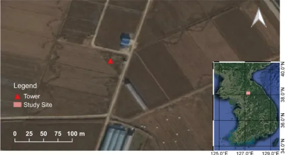
Our study site was a rice paddy located in Cheorwon, Gangwon province, South Korea (38.2013°N, 127.2506°E) registered in the Korea Flux Network (KoFlux) (Figure 1). The region experiences a continental climate with hot humid summers and cold dry winters, which allows for only one growing season per year. In 2016, the mean annual temperature was 11.2 ℃; the lowest temperature was -12.2 ℃ in January and the highest temperature was 31.0 ℃ in August (Korea Meteorology Administration). Annual precipitation was 1180.9 mm, of which two-thirds typically falls during the monsoon period from June to August (Korea Meteorology Administration).
Figure 1. Location of study site and observation tower.
In the rice paddy, the predominant species was Oryza sativa L. ssp. Japonica Odea1 and it was grown intermittently irrigated, with a water depth of about 5 cm.
7
Soil fertilization only occurred once along with transplantation; 12.02 g N m-2 fertilizer was applied at a ratio of 18:7:9 (nitrogen: phosphoric acid: potassium). The entire growing season in 2016 lasted for around four months, from transplantation at the end of April [Day of Year (DOY), 120] to harvest in early September (DOY, 248) (Huang et al. 2018). The phenology of rice is commonly divided into three growth phases: vegetative (DOY 120 to 180); reproductive (DOY 180 to 220); and ripening (DOY 220 to harvest) (Maclean et al. 2013). The vegetative phase is characterized by a gradual increase in leaf emergence and plant height. The reproductive phase is characterized by culm elongation and a decline in tiller number. The ripening phase starts at flowering and ends when the grain is mature to be harvested. During the whole growing season, we visited the study site every one to two weeks, 14 times in total.
2.2. Sun-induced Chlorophyll Fluorescence
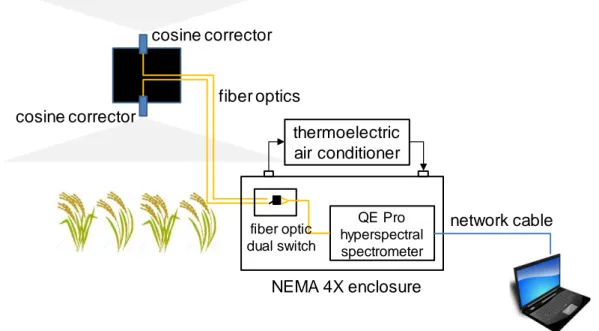
To continuously measure the canopy spectrum for SiF retrieval, we deployed an automated field spectroscopy system (Figure 2). The system includes as main parts a QE Pro spectrometer, two fiber optics and a 2×2 fiber optic dual switch (all components from Ocean Optics, Dunedin, FL, USA). The spectrometer covers the spectral range of 730–790 nm, with a spectral resolution of 0.17 nm, a spectral sampling interval of 0.07 nm, and a signal to noise ratio of around 1000. To avoid dark current drift, the spectrometer was housed in a National Electrical Manufacturers Association 4X enclosure, which was equipped with a thermoelectric air conditioner (400 BTU (DC); EIC Solutions, Warminster, PA, USA) and desiccant, keeping the internal temperature at 25 ℃ and the humidity mostly at a low level. Two fiber optics, pointing toward the zenith (sky) and nadir (rice canopy) directions, respectively, were mounted at around 5 m above the canopy and connected with the spectrometer through the fiber optic dual switch.
8
Both optics were equipped with cosine correctors (CC-3; Ocean Optics, Dunedin, FL, USA) to measure bi-hemispheric irradiance. While the downward field-of-view therefore also included the light-weight tower structure, we assume that its contribution to the total footprint is minimal and that the only effect is a small underestimation of retrieved SiF. Using a custom-written software based on Omni Driver development kits (Ocean Optics, Dunedin, FL, USA), we sequentially recorded upward and downward readings every 10 s from 06:00 to 18:00 (local solar time), and corrected for dark currents and CCD detector nonlinearity for each reading pair. Dark current correction was conducted using values from permanently dark detector pixels. We verified that dark current did not show clear spectral variation and the use of the dark pixels was therefore justified.
Several strategies were applied to assure high data quality. Following the standard method proposed by the spectrometer manufacturer, we conducted spectral calibrations using an HG-1 Mercury Calibration Source (Ocean Optics, Dunedin, FL, USA) before installing the system. Furthermore, radiometric calibration was conducted with an HL-2000-CAL Light Source (Ocean Optics, Dunedin, FL, USA) in the field around every one to two weeks. Next to the QE Pro spectrometer, we installed another spectrometer system (based on Jaz spectrometers; Ocean Optics, Dunedin, FL, USA) to record the sky and the canopy spectrum within the spectral range of 350–1033 nm. We double checked the reliability of QE Pro measurements by frequently comparing averaged downwelling and upwelling irradiance over 730-780 nm from QE Pro and Jaz.
9
Figure 2. Schematic of the canopy SiF observation system.
We retrieved SiF values in the spectral range of 745 to 780 nm using the singular vector decomposition method (SVD) (Guanter et al. 2012; Guanter et al. 2013) (a detailed explanation is provided in the Supplementary Materials A). The fiber optic dual switch appeared to be the cause of a small spectral shift between irradiance spectra from the two fiber optics. To eliminate the influence of this spectral shift as well as artefacts due to high humidity on SiF retrieval, we used the SVD method with appropriate training data and a broad wavelength range. SiF in this study was calculated in units of irradiance based on the bi-hemispheric observation system and reported at 760 nm. We calculated LUEf in the unit of μmol photon emitted @760nm / μmol photon absorbed @400-700nm based on the quantum nature of the physical process of fluorescence emission where one absorbed photon can lead to an emitted fluorescence photon. Daily mean SiF and LUEf were calculated as average of the half hourly values from 08:00 to 18:00 local time. QE Pro hyperspectral spectrometer thermoelectric air conditioner cosine corrector cosine corrector fiber optics NEMA 4X enclosure fiber optic dual switch network cable
10
2.3. Eddy Flux Tower
To quantify gross primary productivity (GPP), we installed a closed-path eddy covariance (EC) system at 9 m above the ground, and processed the data based on the KoFlux data processing protocol. The EC system consists of a three-dimensional sonic anemometer (Model CSAT3, Campbell Scientific Inc., Logan, UT, USA) and a closed-path infrared gas analyzer (Model LI-7200, LI-COR Inc., Lincoln, NE, USA). During the growing season, the peaks of the footprint were located about 30 m south- and northwest of the tower location, while the 80% (50%) contribution to the footprint came from distances within 300 m (100 m) from the tower during the day according to analysis using Kljun et al. (2015)'s flux footprint prediction model. To improve the data quality by eliminating undesirable data, the collected data were examined by the quality control (QC) procedure based on the KoFlux data processing protocol (Hong et al. 2009). This procedure includes the coordinate rotation (double rotation; (Mcmillen 1988)), frequency response correction (Fratini et al. 2012; Horst and Lenschow 2009), humidity correction of sonic temperature (Van Dijk et al. 2004), steady state/developed turbulent condition test (Mauder and Foken 2011), and random sampling error estimation (Finkelstein and Sims 2001). These methods were applied using EddyPro (Version 6, LI-COR Inc.) and additional QC including storage flux calculation and spike detection (Papale et al. 2006) were conducted using the KoFlux standardized data processing program (Hong et al. 2009).
After QC, the final percentage of the data retained was 48.5% for the study period. The data gaps were mostly caused by the unsatisfactory conditions for EC measurement during the nighttime and early morning (e.g., non-steady states and unfavorable developed turbulent conditions). The
11
missing data were gap-filled using a marginal distribution sampling method (Reichstein et al. 2005). For nighttime CO2 flux correction and its partitioning into into GPP and ecosystem respiration (RE), we applied the friction velocity (u*) correction method with the modified moving point test method for determining u* threshold (Kang et al. 2016; Kang et al. 2017) and extrapolated nighttime values of RE into the daytime values using the RE equation (Lloyd and Taylor 1994) with a short-term temperature sensitivity of RE from the nighttime data (Reichstein et al. 2005). The gap-filling and partitioning methods were applied for each cultivation period (i.e., before transplanting, rice growing, and after harvest) separately to prevent interference effects. Daily mean GPP was calculated as average of the half hourly values from 08:00 to 18:00 local time.
2.4. Measurements of Meteorological Variables and Absorbed
PAR
Environmental data were continuously collected every half hour (Figure S3). Air temperature (Ta) and relative humidity (RH) were measured at the top of the tower with a commercial instrument (HMP-35, Vaisala, Helsinki, Finland). This data was also used to quantify vapor pressure deficit (VPD). We measured total photosynthetically active radiation (PAR) and diffuse PAR (PARdif) using a quantum sensor (PQS 1; Kipp & Zonen B.V., Delft, The Netherlands) with a custom-made rotating shadow-band. Its prototype was both described and initially tested in previous studies (Michalsky et al. 1986; Michalsky et al. 1988). The value of total PAR was cross checked using incoming shortwave radiation from a CNR4 radiometer (Kipp & Zonen B.V., Delft, The Netherlands). Cloudy days were defined as daily mean fraction of PARdif larger than 50% (Yang et al. 2015).
12
We used three light emitting diode (LED) sensors (Ryu et al. 2010a; Ryu et al. 2014) to measure incoming PAR above the canopy, canopy reflected PAR and transmitted PAR through the canopy, respectively. We made three sets of the LED sensor system, and located each set in the footprint of the flux tower. The absorbed PAR (APAR) was then calculated as:
APAR = 𝑃𝐴𝑅𝑖𝑛𝑐𝑜𝑚𝑖𝑛𝑔− 𝑃𝐴𝑅𝑟𝑒𝑓𝑙𝑒𝑐𝑡𝑒𝑑− 𝑃𝐴𝑅𝑡𝑟𝑎𝑛𝑠𝑚𝑖𝑡𝑡𝑒𝑑 (3) We confirmed that neglecting the upwelling flux from below the canopy in Equation 3 is justified using observations from an LAI-2200 instrument (LI-COR Inc., Lincoln, NE, USA) (Figure S4). The average of APAR from three sets of the LED sensor system was used to represent the whole canopy. To remove potential measurement bias introduced by the location of LED sensors, diurnal patterns of measured APAR was adjusted and data gaps were filled with simulations from PROSAIL (Jacquemoud and Baret 1990; Jacquemoud et al. 2009; Verhoef 1984) which agreed with LAI-2200 derived fraction of APAR estimates (a detailed explanation is provided in the Supplementary Materials C). Daily environmental variables were calculated as average of the half hourly values from 08:00 to 18:00 local time.
2.5. Leaf Area Index and Maximum Carboxylation Rate
We quantified leaf area index (LAI) using a destructive approach. In each field trip, three hills of rice were randomly selected, and then all of the leaves from each hill were scanned to calculate green and yellow leaf area. A rice hill is a group of rice plants directly adjacent to each other because the seeds or seedlings were planted together (Kumar 2008). Finally, the LAI was calculated based on the total leaf area per hill and rice hill density per unit area (17.0 hills 𝑚−2).
13
To estimate the maximum carboxylation rate (Vcmax), we measured A/Ci curves using an Li-6400 XT instrument (LI-COR Inc., Lincoln, NE, USA) and fitted the Farquhar-von Caemmerer-Berry model (Farquhar et al. 1980). The same same parametrization, cost function and optimization algorithm as in Dechant et al. (2017) was used for the model fitting. However, all of the four main model parameters were left unconstrained and hence fitted here and the protocol for the steps of CO2 reference in the response curve measurements differed from Dechant et al. (2017). For better seasonal comparison, reported Vcmax was adjusted to 25 ℃ using literature values for activation energies from Knorr (2000) and Von Caemmerer (2000). In each field campaign, more than five sunlit leaves were randomly selected and all measurements were collected before 13:00 (local time) to avoid afternoon stomatal depression.
2.6. Statistical Analysis
Both for linear regression and Pearson correlation a significance threshold of 0.05 was used. The Analysis of Covariance (ANCOVA) toolbox and the fitlm function in MATLAB (MathWorks, Inc) were used to test if the effects of environmental conditions and growth stage on regression coefficients were significant. Negative SiF and GPP data were excluded from the analyses. Besides, outliers of LUEp and LUEf (beyond μ ± 3σ) on each day were also excluded from the diurnal relationship analysis.
14
3. Results
3.1. Seasonal Variations of SiF, GPP, LUE
fand LUE
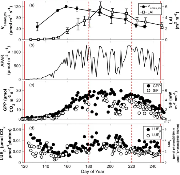
pThe rice canopy showed pronounced seasonal variations in the key structural (LAI) and functional (Vcmax,25) variables (Figure 3a). Leaf Vcmax,25 first increased to 120 μmol 𝑚−2𝑠−1 until DOY 160 and then decreased in the reproductive and ripening phases. Total LAI (including both green, yellow and senescing leaves in the ripening phase) showed a large increase in the vegetative phase with leaf emergence, and reached its maximum value (6 𝑚2𝑚−2) around DOY 180. Subsequently, the LAI slowly decreased in the ripening phase.
Similar seasonal trajectories were observed for SiF and GPP over the whole growing season (Figure 3c). In the seasonal course, daily mean SiF varied from almost 0 to 6 mW m-2 nm-1, and daily mean GPP varied from 0 to around 30 μmol CO2 m-2 s-1. The onset of SiF and GPP occurred on DOY 120, just after rice transplantation. In the vegetative phase, SiF and GPP showed large increases with rice canopy development until approximately DOY 180. During the reproductive phase, SiF and GPP reached their maxima and remained relatively stable except for several days when incoming PAR was low. Both SiF and GPP decreased during the ripening phase (starting approximately at DOY 220) due to leaf senescence until rice harvest. Seasonal variations in APAR explained most of the seasonal variance in SiF and GPP: we found R2 = 0.83 and 0.85 for linear regressions between daily mean APAR with GPP and SiF (Figure 3b, Table 1). The relative RMSEs (RMSE / mean value, rRMSE) were 26% and 31% for GPP and SiF, respectively. The seasonal pattern of SiF revealed a strong linear relationship to that of GPP (R2
15
= 0.87, rRMSE = 25%; Figure 4c). Besides the overall seasonal pattern, SiF also tracked day-to-day GPP variations mostly induced by varying PAR. This can be seen for the decrease of GPP around DOY 201 to 203, for example (Figure 3b, c).
Figure 3. Seasonal variations of measured variables.
(a) Seasonal variations of field measured Vcmax,25 and LAI. Error bar indicates standard deviation of all measured samples. We added one day to DOY of LAI measurement to avoid overlapping with measurement of Vcmax,25; (b) daily mean absorbed photosynthetically active radiation (APAR); (c) daily mean gross primary productivity (GPP) and sun-induced fluorescence (SiF); (d) daily mean light use efficiency of photosynthesis (LUEp) and light use efficiency of fluorescence
16
(LUEf). Two solid red lines indicate start (DOY 120) and end (DOY 247) of the growing season, respectively. Two dashed red lines indicate beginning of reproductive and ripening phases, respectively. Daily mean values were calculated as average of half hourly values from 08:00 to 18:00 local time.
In addition, LUEf also presented a similar seasonal pattern to LUEp (Figure 3d) and a weak positive linear relationship with LUEp (R2 = 0.24, rRMSE = 27%; Table 1). Over the whole growing season, daily mean LUEp varied from 0 to around 0.05 μmol CO2 μmol photon-1, and daily mean LUEf from 0 to 6× 10⁻⁵ μmol photon@760nm μmol-1 photon@400-700nm. The overall seasonal variations of LUEp and LUEf did not show strong relationships with canopy structural variables, but there appears to be a weak correlation to LAI for the time after DOY 150. Peak values of LUEf and LUEp generally appeared on days with low PAR (Figure 3b, d).
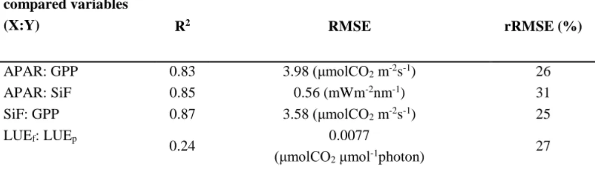
Table 1. Fitting goodness of linear regressions between compared variables on daily mean scale.
The coefficient of determinations (R2), RMSE and relative RMSEs (RMSE / mean value, rRMSE) of fitted linear regressions between compared variables on daily mean scale. All R2 values were statistically significant (p<0.05).
compared variables
(X:Y) R2 RMSE rRMSE (%)
APAR: GPP 0.83 3.98 (μmolCO2 m-2s-1) 26
APAR: SiF 0.85 0.56 (mWm-2nm-1) 31
SiF: GPP 0.87 3.58 (μmolCO2 m-2s-1) 25
LUEf: LUEp
0.24 0.0077
(μmolCO2 μmol-1photon)
27
3.2. Relationships Between SiF and GPP for Different
Environmental Conditions and Phenological Stages
17
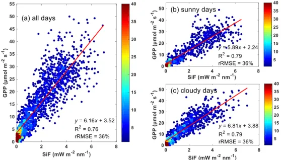
A strong linear relationship was found between half hourly SiF and GPP over the whole growing season (R2 = 0.76, rRMSE = 36%; Figure 4a). Considering measurements only on sunny or cloudy days showed stronger linear relationships with higherR2 and lower rRMSE (R2 = 0.79, rRMSE = 36% for both sunny and cloudy days; Figure 4b, c). Furthermore, compared with sunny days, the linear regression on cloudy days had a significantly steeper slope of GPP to SiF (slope = 5.89 ± 0.22 for sunny days; and slope = 6.81 ± 0.22 for cloudy days, uncertainty indicates 95% CI, Figure 4b, c). The significant differences in slopes between sunny and cloudy were also observed when forcing the linear regression to pass the origin (R2 = 0.77, slope = 6.53 ± 0.14 for sunny days; and R2 = 0.74, slope = 8.18 ± 0.16 for cloudy days).
Figure 4. Scatter plots and linear regressions (𝑦 = a × 𝑥 + 𝑏) between half hourly SiF and GPP.
(a) all illumination conditions; (b) sunny days only; and (c) cloudy days only. Linear regression lines are shown in red and regression statistics are given. R2 and rRMSE represent the coefficient of determination and the relative RMSE (RMSE / mean) of fitted linear regressions, respectively. Color map represents point density.
18
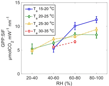
The ratio of GPP to SiF showed a significant increasing trend with RH (ANCOVA p < 0.05, Figure 5). For a more detailed analysis, SiF and GPP data were separated according to certain ranges of Ta and RH values. In 13 out of 14 cases with available data, the linear regression fitted half hourly values of SiF and GPP well (p < 0.05; Table S2), with low uncertainty in individual slope values (Figure 5). Moreover, regressions results indicated that even within the relatively narrow ranges of Ta values, RH significantly impacted the slope between GPP and SiF (GPP: SiF in Figure 6), and the slope generally increased with higher RH values.
Figure 5. Slope of the linear regressions between half hourly SiF and GPP under different environmental conditions.
Slope of the linear regressions (y=a×x) symbolized by GPP: SIF between half hourly SiF and GPP over different air temperature (Ta) and relative humidity (RH) values. Uncertainty indicates 95% CI.
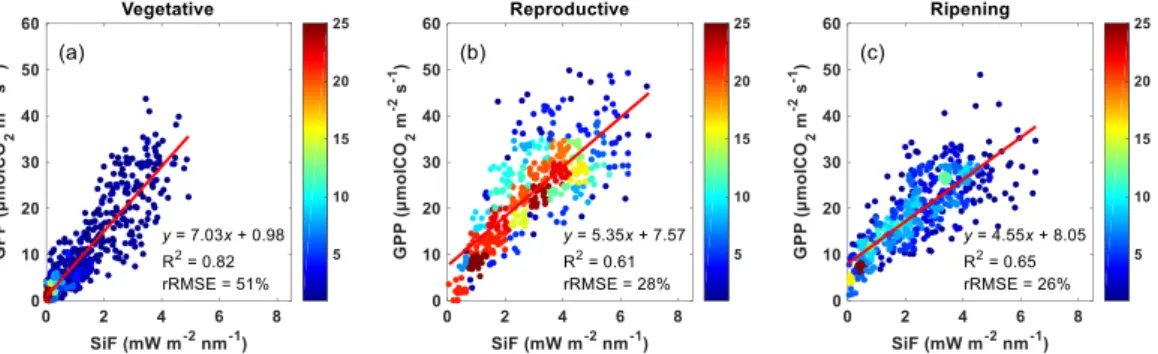
We analyzed the effect of the growth stage on the SiF-GPP relationship and found significant effects (Figure 6). Both slopes and offsets of the linear regression
19
differed significantly (ANCOVA p < 0.05) between growth stages with slope values showing decreasing and intercept values increasing trends over time. The largest part of the variance was explained for the vegetative stage (R2=0.82, Figure 6a), the lowest for the reproductive stage (R2=0.61, Figure 6b) and intermediate values for the ripening stage (R2=0.65, Figure 6c).
Figure 6. SiF-GPP relationships for the vegetative, reproductive and ripening growth stages of rice.
SiF-GPP relationships for the vegetative, reproductive and ripening growth stages of rice. Linear regression lines are shown in red and regression statistics are given. R2 and rRMSE represent the coefficient of determination and the relative RMSE (RMSE / mean) of fitted linear regressions, respectively. Color map represents point density.
In order to confirm that there were indeed significant effects of RH, PARdif proportion and growth stage despite some correlation between them, we conducted a multiple regression analysis to estimate GPP from SiF including all relevant explanatory variables and interactions. The choice of the latter was based on mechanistic considerations such as the drivers of stomatal conductance (Ball et al. 1987) and the effects of diffuse radiation on LUEp (Gu et al. 2002; Wit 1965) as well as observations from Figure 6 on the seasonal effects. The main results of this analysis are reported in Table 2 where the analogous analysis with APAR instead of SiF as main predictor is also given. We found similar improvements for single explanatory variables for the interactions of SiF with RH and SiF with PARdif
20
proportion (increase of total growing season R2 from 0.74 to 0.77), while growth stage had a slightly larger effect (increase to R2=0.80). Adding interaction effects of PARdif proportion with SiF to those of RH did only slightly improve the results despite the significance of all terms.
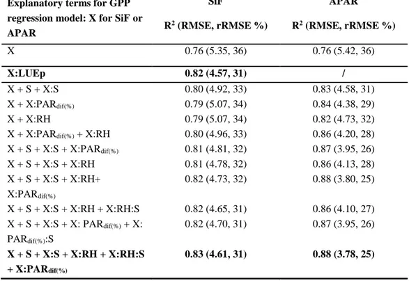
Table 2. Overview of regression models for GPP estimation from half-hourly data including relevant environmental variables and phenology.
The latter is incorporated in the form of growth stage (S) with three factor levels and environmental variables are relative humidity (RH) and diffuse PAR ratio (PARdif(%)).The plus sign indicates additive terms while the colon indicates interaction terms. R2 and rRMSE represent the coefficient of determination and the relative RMSE (RMSE / mean) of fitted regressions models, respectively. The best models based on either environmental predictors or LUEp are highlighted in bold.
Explanatory terms for GPP regression model: X for SiF or APAR
SiF APAR
R2 (RMSE, rRMSE %) R2 (RMSE, rRMSE %)
X 0.76 (5.35, 36) 0.76 (5.42, 36) X:LUEp 0.82 (4.57, 31) / X + S + X:S 0.80 (4.92, 33) 0.83 (4.58, 31) X + X:PARdif(%) 0.79 (5.07, 34) 0.84 (4.38, 29) X + X:RH 0.79 (5.07, 34) 0.82 (4.73, 32) X + X:PARdif(%) + X:RH 0.80 (4.96, 33) 0.86 (4.20, 28) X + S + X:S + X:PARdif(%) 0.81 (4.81, 32) 0.87 (3.95, 26) X + S + X:S + X:RH 0.81 (4.78, 32) 0.86 (4.13, 28) X + S + X:S + X:RH+ X:PARdif(%) 0.82 (4.73, 32) 0.88 (3.80, 25) X + S + X:S + X:RH + X:RH:S 0.82 (4.65, 31) 0.86 (4.10, 27) X + S + X:S + X: PARdif(%) + X: PARdif(%):S 0.82 (4.70, 31) 0.87 (3.95, 26) X + S + X:S + X:RH + X:RH:S + X:PARdif(%) 0.83 (4.61, 31) 0.88 (3.78, 25)
The effect of growth stage alone was slightly larger than for RH and PARdif proportion. Combining the effects of the latter with growth stage further improved the results up to an R2 value of 0.81, which was linked to about 14% reduction in
21
the GPP estimation error (RMSE) compared to the model based exclusively on SiF. While the corresponding results for APAR as main predictor were generally similar, PARdif proportion seemed to have a slightly bigger effect compared to RH and the overall error reduction was considerably larger (about 30%). For all cases with additional predictors, the APAR-based models showed better performance than the corresponding SiF-based models. The discrepancy in GPP estimation error between the best SiF- and APAR-based models was considerable (rRMSE of 31% and 25%, respectively), while the difference in RMSE for the simplest models was small (< 1%). Furthermore, we also found that the model based on the product of SiF with LUEp outperformed the best SiF-based model with environmental and growth stage interaction terms. If not indicated otherwise in the tables, all interaction terms were significant. We used the Akaike information criterion (AIC) to verify that the improvement obtained by adding more predictor terms to the models was not offset by the corresponding reduction in degrees of freedom (results not shown).
3.3. Diurnal Relationships Between SiF and GPP
On the diurnal scale for individual date, SiF showed linear relationships with GPP over two thirds of individual days over the growing season (Figure 7c), and their relationships were predominantly driven by APAR (Figure 7a, b). We analyzed the diurnal relationships between APAR and GPP, APAR and SiF, SiF and GPP, as well as LUEf and LUEp on individual days over the whole growing season. Only days with more than 50% observations from 08:00 to 18:00 local time were considered. Among 126 available days, GPP showed significant linear relationships to APAR on 81% of individual days (R2: 0.19-0.96, Figure 8a). More than 70% of the days that had no significant APAR-GPP relationship occurred in the early stages of the growing season (DOY <143), which was characterized by
22
low numbers of available GPP measurements per day. Over the whole growing season, 90 days were available for SiF data. Around 84% of those days showed significant linear APAR-SiF relationships (Figure 8b), which was a slightly higher fraction than that for GPP, and their R2 ranged from 0.20 to 0.98. The mean R2 over days with significant relationship was 0.65 for GPP, and 0.76 for APAR-SiF. Furthermore, we found significant linear relationships between SiF and GPP on around 70% of individual days (Figure 8c), and their R2 ranged from 0.19 to 0.92, with a mean value of 0.60.
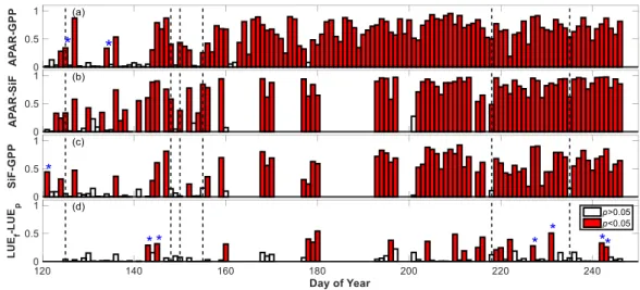
Figure 7. Coefficients of determinations (R2) of linear regressions (𝑦 = a × 𝑥 + b) between half-hourly measurements.
(a) APAR and GPP; (b) APAR and SiF; (c) SiF and GPP; and (d) LUEf and LUEp on individual days over the whole growing season. Vertical dashed lines represent individual days when SiF is not significantly related to GPP, while both SiF and GPP show significant linear relationships with APAR. Blue ‘*’ indicates negative correlations between compared variables.
Among 90 available days for SiF and GPP, 27 days of them presented no significant linear relationship between SiF and GPP (Figure 8c). Most of these instances (74%) were from days before DOY 150 which also showed no significant relationships between APAR with either GPP or SiF. Besides, there were cases for which even though both SiF and GPP were linearly related to APAR, the absence
23
of strong relationships between LUEf and LUEp seemed to lead to weak SiF-GPP relationships (see individual days with vertical dashed lines in Figure 8). Over the whole growing season, LUEf only showed linear relationships with LUEp on around 22% of individual days (p < 0.05, Figure 8d), and their R2 ranged from 0.19 to 0.54, with a mean value of 0.34. In addition, on around one third of the days with significant relationships, LUEf showed negative relationships with LUEp.
3.4. Relationships Between LUE
fand LUE
pon Clear Sky Days
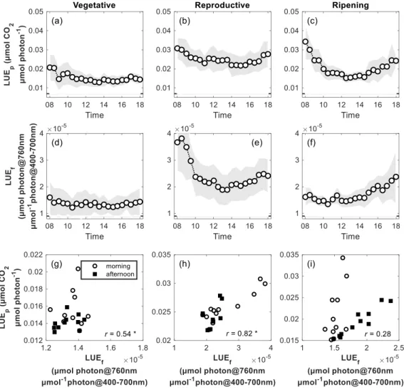
To investigate the effects of phenology on LUEf and LUEp relationships, clear sky days (daily mean proportion of beam direct PAR > 0.7) from three growth phases were chosen (10, 12, 8 days in vegetative, reproductive and ripening phases, respectively), and the mean diurnal courses of LUEf and LUEp were calculated (Figure 8a–f). We then analyzed diurnal correlations between LUEf with LUEp (Figure 8g–i) over different phenological phases. Across the three growth phases, LUEp followed a typical diurnal cycle under clear sky conditions, where values showed a steady decrease during morning hours and a subsequent increase after solar noon (13:00 local time) (Figure 8a–c). In the vegetative and reproductive phases, we observed qualitatively similar diurnal courses for LUEf and LUEp (Figure 8d, e), which decreased from early in the morning until solar noon, and slowly increased afterwards. Significant LUEf-LUEp relationships were observed in the vegetative (r = 0.54) and reproductive (r = 0.82) phases (Figure 8g–i). In the ripening phase, LUEf and LUEp showed decoupled diurnal variations: in contrast to LUEp, the diurnal course of LUEf was highly asymmetric with almost constant values in the morning and showed qualitatively similar behavior as LUEp only in the afternoon (Figure 8c). This resulted in an overall non-significant relationship between LUEf and LUEp in the ripening stage, while the relationship for only the afternoon hours was strong (r =0.95) and significant (Figure 8i).
24
Figure 8. Averaged diurnal courses on clear sky days (daily mean direct PAR proportion > 0.7).
(a-c) LUEp and (d–f) LUEf (circles represent averaged values, and shaded bands represent standard deviation), as well as correlations between averaged LUEp and LUEf over the whole day at different growing stages (g–i). In (g–i), ‘r’ denotes Pearson correlation. From left to right, each column represents vegetative, reproductive, and ripening phase, respectively.
To understand the relationships of LUEf and LUEp with relevant environmental variables across different phenological stages, we applied partial correlation analysis for half-hourly APAR, PARdif proportion, and VPD data on the dates that were used in Figure 8. In contrast to LUEf, LUEp was significantly and
25
positively correlated to PARdif proportion in all phenological stages. LUEf showed significant negative correlations to APAR except for the vegetative stage where the correlation was positive. In the ripening stage, a significant positive correlation was found between VPD and LUEf, while the correlation was always negative for LUEp in all the three growing stages.
Table 3. Partial correlations between LUE and the environmental variables. Partial correlations between half-hourly LUE (LUEp or LUEf) and the environmental variables: absorbed PAR (APAR), diffuse PAR proportion, and vapor pressure deficit (VPD) between 0800hh and 1800hh on clear sky days (daily mean direct PAR proportion > 0.7). Bold font indicates significant correlation (p <0.05).
Growing phase APAR Diffuse PAR proportion VPD Vegetative LUEp 0.14 0.11 -0.42 LUEf 0.59 0.17 -0.03 Reproductive LUEp -0.19 0.31 -0.27 LUEf -0.31 0.07 -0.35 Ripening LUEp -0.32 0.58 -0.12 LUEf -0.23 0.20 0.53
26
4. Discussion
In this study, we retrieved SiF values from automatic ground-based observations and investigated the relationships between canopy SiF and GPP from eddy covariance measurements at seasonal and diurnal scales in a rice paddy. More importantly, we analyzed how environmental conditions influenced the relationship between SiF and GPP, as well as explored the response of LUEf and LUEp to environmental variations at different rice phenological stages. We believe this is the first study that reported continuous observations of GPP and SiF over the whole growing season in rice paddy.
4.1. Relationships Between SiF and GPP on Different Temporal
Scales
At the seasonal scale, daily mean SiF tracked temporal variations of daily mean GPP well (Figure 3c), and showed a strong linear relationship with GPP, which is comparable to APAR (R2 = 0.83, rRMSE = 26% for APAR-GPP; R2 = 0.87, rRMSE = 25% for SiF-GPP. Table 1). This finding demonstrated that the linear relationship between seasonal patterns of SiF and GPP was mostly explained by the strong APAR-SiF relationship (R2 = 0.85, Table 1), which is similar to the result of Yang et al. (2015) who observed higher SiF-APAR (R2 = 0.79) than SiF-GPP (R2 = 0.73) correlation. Nevertheless, we also found a weak but significant relationship between daily mean of LUEf and LUEp over the growing season (p < 0.05, R2 = 0.24, Figure 3d, Table 1). This finding is consistent with Yang et al. (2015) that found a slightly higher correlation at daily temporal resolution (R2 = 0.38). Rossini et al. (2010), however, found a strong linear relationship between LUEf and LUEp (R2 = 0.74) in a rice paddy with data from 15 measurement campaigns over two years, and demonstrated that this relationship could be used to considerably improve LUE-based GPP models.
27
On the diurnal scale, we found that SiF was linearly related with GPP on more than two thirds of individual days, with a mean R2 value of 0.60 (Figure 7c). Besides, similar to the seasonal scale, the SiF-GPP relationship on the diurnal scale was also predominantly explained by APAR (Figure 7). In general, APAR performed slightly better than SiF in tracking diurnal variations in GPP, which had more days with significant linear relationships (81% for APAR-GPP, and 70% for SiF-GPP) and a slightly higher mean value of explained variance (R2 = 0.65 and 0.60 for APAR and SiF, respectively). Moreover, the significant linear relationships between LUEf and LUEp were only found on 22% with a rather low mean value (R2=0.34). The higher correlation of LUEf and LUEp at the seasonal scale with daily temporal resolution implies that the effects of more seasonally varying properties such as pigment contents, photosynthetic capacity and canopy structure on LUEp is better captured by SiF than the effects of short-term variations of environmental conditions on LUEp. The poorer performance of SiF to track GPP in the early growing stage might be associated with the decoupled diurnal variation of LUEf and LUEp in most of the days (> 80%) (Figure 7d).
While both model simulations and ground based observations have demonstrated that relationships between SiF and GPP tend to be more linear at coarser temporal scale (Damm et al. 2015; Goulas et al. 2017; Zhang et al. 2016b), we found that the linear relationships between half hourly SiF and GPP were comparable to the corresponding daily relationships (R2 = 0.76 for half hourly SiF and GPP, Figure 4a; R2 = 0.87 for daily mean SiF and GPP, Table 1). Zhang et al. (2016b), for instance, reported that the R2 of the linear regression between SiF-GPP at the Harvard Forest increased from 0.42 over 0.74 to 0.84 after aggregating from hourly over daily to 16-days. Both results are not contradictory when considering the variation of GPP to APAR. The linearization effect is caused
28
mainly by the decrease of APAR values due to averaging such that the saturation effects for GPP tend to get weaker or even entirely disappear (Damm et al. 2015; Zhang et al. 2016b), which is in accordance with well-known observations that temporal averaging tends to linearize the response between GPP and APAR (Baldocchi and Amthor 2001; Ruimy et al. 1995). However, in the rice paddy, saturation of GPP with APAR and GPP with SiF was not as clearly observed at half hourly time scale (linear regression: R2 = 0.73, rRMSE = 34% for APAR-GPP) as in other studies (e.g. Zhang et al., 2016a). Hence the mechanism of the linearization effect described above could only lead to moderate improvements in the linear SiF-GPP relationship on daily scale (R2 = 0.85, rRMSE = 26%) that were comparable to the change from daily to 16 day averages in Zhang et al. (2016a). Addition of fertilizer and the erectophile canopy of rice might explain the absence of strong saturation effects of GPP with APAR.
4.2. Effects of Environmental Factors and Phenology on the
Relationship Between SiF and GPP
Half hourly SiF was strongly and linearly related to half hourly GPP over the whole growing season in the rice paddy (R2 = 0.76), but the slope of their linear regressions was found to vary depending on environmental conditions such as PARdif fraction and RH (Figures 4, 5, S4) as well as the growth stage (Figure 6).
We found that sky conditions had two effects on the relationship between SiF and GPP. First, the GPP to SiF ratio was higher on cloudy days (Figure 4b, c). Greater proportion of diffuse light that allows more evenly distributed light over different canopy layers is well known to increase canopy LUEp by enhancing photosynthesis in shaded leaves which are light limited (Alton et al. 2007; Gu et al. 2003). The effects of diffuse light on LUEf should also be considered in this context.
29
According to the escape ratio formula for far-red SiF by Yang and van der Tol (2018), LUEf is expected to increase with PARdif fraction due to the increase in the canopy near-infrared reflectance (e.g. Ryu et al., 2010a) while the canopy interceptance is not much affected for a closed canopy. This effect, however, would tend to decrease the GPP:SiF ratio on cloudy days, which is not the observed pattern and hence, the LUEp effects seem to dominate over LUEf effects in the response to diffuse light. Second, the linear relationship was stronger considering only sunny or cloudy days separately, while the correlation on sunny and cloudy days are comparable (Figure 4b, c). In contrast to our result, Zhang et al. (2016b) also found that the SiF-GPP relationship became stronger during sunny days in Harvard forest (R2=0.79 for sunny, R2=0.74 for cloudy) and Miao et al. (2018) confirmed this tendency for soybean (R2=0.65 for sunny, R2=0.52 for cloudy). Goulas et al. (2017), however, found that in a winter wheat field the relationship between half-hourly SiF and GPP slightly weakened if measurements under sunny conditions were considered. The canopy structure of a rice paddy, deciduous forest, and winter wheat field differ substantially in terms of LAI and leaf inclination angle but effects of PARdif were observed in all cases. Our multiple regression analysis also confirmed that incorporating PARdif proportion with SiF improved GPP prediction (Table 2). Overall, these findings suggest that at the canopy scale, not only light intensity but also the PARdif fraction should be considered when linking SiF to GPP.
Furthermore, we found that the ratio of GPP to SiF generally increased with RH in the rice paddy (Figure 5). This trend was generally consistent across each phenological stage (data not shown). A C3 leaf biochemical fluorescence model predicted that GPP:SiF ratio increased with RH and Ta (van der Tol et al. 2014) (Figure 9). We used the model with diverse ranges in PAR and Vcmax,25, which all produced increasing trends of the GPP:SiF ratio with RH, which supports our
in-30
situ data. The model results revealed that increase of RH led to higher stomatal conductance, and hence intercellular CO2 concentration, and GPP whereas SiF was relatively insensitive to RH. This implies that GPP:SiF relationship against RH is dominantly controlled by LUEp, not LUEf. Multiple regression analysis also confirmed that combining RH with SiF improved GPP prediction (Tables 2, 3). There is still ongoing debate whether RH or VPD is the direct driver of stomatal limitation of photosynthesis (e.g.) (Sato et al. 2015). We therefore compared multiple regression analyses using either RH or VPD and found consistent results with very small differences. This can also be attributed to the high correlation of RH and VPD for our dataset (R2=0.78).
Figure 9. Simulated leaf-level values of the ratio of photosynthesis (GPP) to sun-induced chlorophyll fluorescence (SiF) against relative humidity and temperature. Data presented here used a C3 leaf biochemical photosynthesis model (van der Tol et al. 2014) at Vcmax,25=80 µmol m-2 s-1, CO2=400 ppm, O2=21%. PAR=1500 µmol m-2 s-1 forsolid lines and PAR = 500 µmol m-2 s-1 for dashed lines.
31
We found clear evidence of a seasonally changing SIF-GPP relationship (Figure 6), which could be related to canopy structure effects affecting the fraction of emitted SiF escaping the canopy. Recently published results including both simulations and field observations showed strong effects of canopy structure on the APAR-SiF relationship (Du et al. 2017), which in turn will also affect the GPP-SiF relationship. In the rice paddy, mean leaf inclination angle, which was measured using a leveled digital camera photography method (Ryu et al. 2010b), changed in the course of the growing season with variations from 50 to 70 degrees (data not shown) and this together with changes in LAI as well as leaf senescence in the ripening stage is expected to affect the fraction of SiF escaping the canopy. Multiple regression analysis confirmed that incorporating phenological stage information into SiF improved GPP predictions (Tables 2, 3). Therefore, accounting for the escape fraction that depends on canopy structure may be necessary to improve SiF-based GPP estimation. Recently, a simplified approach to calculate the escape fraction was presented by Yang and van der Tol (2018) that seems promising for future application. Furthermore, anisotropy effects have been shown to play a role also for SiF (Liu et al. 2016; Pinto et al. 2017). While a study of the latter goes beyond the scope of our work, they should be addressed in more detail in the future.
4.3. Effects of Environmental Factors and Phenology on Light
Use Efficiencies on Clear Sky Days
Studying the relationships of LUEf and LUEp on clear sky days is important as airborne campaigns are typically conducted on such days and satellite data acquired on cloudy days tend to suffer from data quality limitations. LUEf and LUEp responded differently to APAR and VPD on clear sky days across vegetative, reproductive, and ripening stages (Table 3). We found that LUEf showed positive
32
correlation to APAR only in the vegetative stage while correlations were negative in the other stages (Table 3). Leaf level simulation using the SiF leaf model (van der Tol et al. 2014) implemented in the widely used SCOPE model (van der Tol et al. 2009) reported that LUEf increased then decreased with APAR, and with greater Vcmax,25, the inflection point moved towards right (i.e. higher APAR) (Frankenberg and Berry 2018; van der Tol et al. 2014). In the vegetative stage, Vcmax,25 approached peak values around 120 μmol m-2 s-1 and APAR was relatively lower than the other stages (Figure 3). We assume the higher Vcmax,25 with lower APAR led to the positive correlation between LUEf and APAR (Figure 3, Table 3). In the reproductive and ripening stages, Vcmax,25 gradually decreased while keeping a high level of APAR, which is likely to explain the negative correlations between LUEf and APAR. The photosynthesis model based on Farquhar et al. (1980) and Collatz et al. (1991) implemented in SCOPE predicted a consistent decrease of LUEp with APAR regardless of Vcmax,25 values. This agreed very well with our result that LUEp was negatively correlated to APAR across all phenological stages that experienced a large seasonal variation in Vcmax,25 (Table 3, Figure 3a). While the latter finding is expected to also hold at the canopy level (Knohl and Baldocchi 2008), the apparently good agreement of leaf-level LUEf -APAR relationships with canopy observations is somewhat surprising as the low APAR values at the beginning of the season are due to low overall LAI and not due to low APAR for individual leaves. That is, individual leaves might be light saturated, which implies mostly negative correlation of LUEf with APAR at the leaf-level. Therefore, an overall negative correlation of LUEf with APAR might also be expected at the canopy level. Further experimental studies and simulations are needed to investigate this.
We found VPD was positively correlated only to LUEf in the ripening stage (Table 3). The LUEp:LUEf ratio substantially decreased in the afternoon of the ripening stage (Figure 8i) indicating that, relatively speaking, the rice canopy
33
converted a larger proportion of APAR into SiF than it used for photochemical reactions compared to the morning hours. In the ripening stage, low values of Vcmax,25 and greater VPD in the afternoon would lead more of the absorbed energy to be dissipated in processes other than photosynthesis such as NPQ and fluorescence. Diurnal hysteresis effects involving changes in the LUEp:LUEf ratio were previously reported (Porcar-Castell et al. 2014), although with lower LUEf in the afternoon in contrast to our findings. However, leaf senescence was shown to affect LUEp and NPQ in previous studies (Lu et al. 2001; Wingler et al. 2004) and this might also affect the diurnal relationships. We are cautious in our interpretation as the canopy includes up to 30% yellow leaves in the ripening stage (data not shown), which still partly contribute to APAR but do not play any direct role in photochemistry, fluorescence and NPQ. However, they can contribute to changes in the SiF escape fraction and thus modify the effective LUEf, which could not be corrected for with our observations.
4.4. Synthesis and Implications of Statistical Analysis of
APAR-GPP, SiF-GPP and LUE
p-LUE
fRelationships
Overall, we found that for 30 min temporal resolution, APAR-based models outperformed SiF-based models for GPP estimation in all cases, both for the whole growing season (Table 2) and for the separate growth stages (results not shown). Furthermore, the improvements when including environmental and growth stage effects were substantially larger for APAR-based than SiF-based models (Tables 2 and 3). In addition, we found that the LUEf -LUEp relationship was very weak at high temporal resolution and that using the product of SiF with LUEp rather than SiF directly considerably decreased the GPP estimation errors (Tables 2, 3). The above-mentioned findings all suggest that SiF observed in the rice paddy should be considered primarily as proxy for APAR rather than a more direct link to
34
photosynthesis that contains considerable information on LUEp. This is consistent with the experimental results of Miao et al. (2018) for soybean that reported stronger relationships between SiF and APAR than SiF and GPP at half-hourly temporal resolution. All these findings seem to contradict other studies that reported canopy escaping SiF as proxy for photosynthetic electron transport rate (ETR), which is the product of APAR with the efficiency of photosystem II (Guan et al. 2016; Zhang et al. 2014).
Our results have important implications for SiF-based GPP estimation at large scales. From the observation that canopy-level retrieved SiF in the rice paddy contains almost exclusively information on APAR, it follows that the SiF-GPP relationship corresponds to the APAR-GPP relationship and hence needs to be modified for well-known LUEp effects related to RH or VPD, PARdif, temperature and phenology (Jenkins et al. 2007; Knohl and Baldocchi 2008; Running et al. 2004). Satellite remote sensing enables us to monitor those key variables such as PARdif proportion (Figure 4) (Ryu et al. 2018), RH (Figure 5) (Hashimoto et al. 2008; Ryu et al. 2008), and phenology information (Figure 6) such as LAI, clumping index, and mean leaf angle (He et al. 2016; Myneni et al. 2002; Zou and Mõttus 2015) across multiple spatial and temporal scales, which offers new opportunities for monitoring GPP through SiF and LUEp.
35
5. Conclusion
We investigated the relationships of SiF retrieved from high-resolution spectrometer observations with GPP over an entire growing season in a rice paddy. We found strong linear relationships between SiF and GPP both at half-hourly and daily temporal resolutions, but that these were almost exclusively driven by the strong relationships between SiF and APAR. On the diurnal scale, the SiF-APAR relationships were considerably stronger than the SiF-GPP relationships. The relationships between LUEf and LUEp were generally weak and inconsistent on both seasonal and diurnal scales at high temporal resolution, but showed clear dependence on environmental factors as well as plant phenology on clear sky days. We demonstrated that including effects of RH and the diffuse PAR fraction as well as growth stage into statistical models of SiF- and APAR-based GPP estimation considerably improved the performance. This is consistent with commonly used approaches to model photosynthetic light use efficiency based on environmental variables and indicates that at least at high temporal resolution, canopy-level SiF for rice is essentially only a good proxy for APAR and does not contain much relevant information on LUEp. This has important implications for future studies aiming at using SiF information to improve large scale GPP estimation, no matter if process-based or empirical approaches are applied.
36
References
Alton, P.B., North, P.R., & Los, S.O. (2007). The impact of diffuse sunlight on canopy light‐use efficiency, gross photosynthetic product and net ecosystem exchange in three forest biomes. Global Change Biology, 13, 776-787
Baker, N.R. (2008). Chlorophyll Fluorescence: A Probe of Photosynthesis In Vivo.
Annual Review of Plant Biology, 59, 89-113
Baldocchi, D.D., & Amthor, J.S. (2001). Canopy photosynthesis: history. Terrestrial
Global Productivity; Academic Press: New York, NY, USA, 9-31
Ball, J.T., Woodrow, I.E., & Berry, J.A. (1987). A model predicting stomatal conductance and its contribution to the control of photosynthesis under different environmental conditions. Progress in photosynthesis research (pp. 221-224): Springer Buschmann, C., Langsdorf, G., & Lichtenthaler, H.K. (2000). Imaging of the blue, green, and red fluorescence emission of plants: An overview. Photosynthetica, 38, 483-491 Cheng, Y.B., Middleton, E.M., Zhang, Q.Y., Huemmrich, K.F., Campbell, P.K.E., Corp, L.A., Cook, B.D., Kustas, W.P., & Daughtry, C.S. (2013). Integrating Solar Induced Fluorescence and the Photochemical Reflectance Index for Estimating Gross Primary Production in a Cornfield. Remote Sensing, 5, 6857-6879
Christian, F., B., F.J., John, W., Grayson, B., S., S.S., Jung‐Eun, L., C., T.G., André, B., Martin, J., Akihiko, K., & Tatsuya, Y. (2011). New global observations of the terrestrial carbon cycle from GOSAT: Patterns of plant fluorescence with gross primary
productivity. Geophysical Research Letters, 38
Collatz, G.J., Ball, J.T., Grivet, C., & Berry, J.A. (1991). Physiological and
Environmental-Regulation of Stomatal Conductance, Photosynthesis and Transpiration - a Model That Includes a Laminar Boundary-Layer. Agricultural and Forest
Meteorology, 54, 107-136
Damm, A., Guanter, L., Paul-Limoges, E., van der Tol, C., Hueni, A., Buchmann, N., Eugster, W., Ammann, C., & Schaepman, M.E. (2015). Far-red sun-induced chlorophyll fluorescence shows ecosystem-specific relationships to gross primary production: An assessment based on observational and modeling approaches. Remote Sensing of
Environment, 166, 91-105
Dechant, B., Cuntz, M., Vohland, M., Schulz, E., & Doktor, D. (2017). Estimation of photosynthesis traits from leaf reflectance spectra: Correlation to nitrogen content as the dominant mechanism. Remote Sensing of Environment, 196, 279-292
37
Du, S.S., Liu, L.Y., Liu, X.J., & Hu, J.C. (2017). Response of Canopy Solar-Induced Chlorophyll Fluorescence to the Absorbed Photosynthetically Active Radiation Absorbed by Chlorophyll. Remote Sensing, 9, 911
Farquhar, G.D., von Caemmerer, S., & Berry, J.A. (1980). A biochemical model of photosynthetic CO2 assimilation in leaves of C3 species. Planta, 149, 78-90 Finkelstein, P.L., & Sims, P.F. (2001). Sampling error in eddy correlation flux measurements. Journal of Geophysical Research-Atmospheres, 106, 3503-3509
Flexas, J., Briantais, J.M., Cerovic, Z., Medrano, H., & Moya, I. (2000). Steady-state and maximum chlorophyll fluorescence responses to water stress in grapevine leaves: A new remote sensing system. Remote Sensing of Environment, 73, 283-297
Frankenberg, C., & Berry, J. (2018). Solar Induced Chlorophyll Fluorescence: Origins, Relation to Photosynthesis and Retrieval. Reference Module in Earth Systems and
Environmental Sciences: Comprehensive Remote Sensing (pp. 143-162). Oxford:
Elsevier
Fratini, G., Ibrom, A., Arriga, N., Burba, G., & Papale, D. (2012). Relative humidity effects on water vapour fluxes measured with closed-path eddy-covariance systems with short sampling lines. Agricultural and Forest Meteorology, 165, 53-63
Goulas, Y., Fournier, A., Daumard, F., Champagne, S., Ounis, A., Marloie, O., & Moya, I. (2017). Gross Primary Production of a Wheat Canopy Relates Stronger to Far Red Than to Red Solar-Induced Chlorophyll Fluorescence. Remote Sensing, 9, 97
Gu, L., Baldocchi, D., Verma, S.B., Black, T., Vesala, T., Falge, E.M., & Dowty, P.R. (2002). Advantages of diffuse radiation for terrestrial ecosystem productivity. Journal of
Geophysical Research: Atmospheres, 107
Gu, L., Baldocchi, D.D., Wofsy, S.C., Munger, J.W., Michalsky, J.J., Urbanski, S.P., & Boden, T.A. (2003). Response of a deciduous forest to the Mount Pinatubo eruption: enhanced photosynthesis. Science, 299, 2035-2038
Guan, K., Berry, J.A., Zhang, Y., Joiner, J., Guanter, L., Badgley, G., & Lobell, D.B. (2016). Improving the monitoring of crop productivity using spaceborne solar-induced fluorescence. Globle Change Biology, 22, 716-726
Guanter, L., Frankenberg, C., Dudhia, A., Lewis, P.E., Gómez-Dans, J., Kuze, A., Suto, H., & Grainger, R.G. (2012). Retrieval and global assessment of terrestrial chlorophyll fluorescence from GOSAT space measurements. Remote Sensing of Environment, 121, 236-251
Guanter, L., Rossini, M., Colombo, R., Meroni, M., Frankenberg, C., Lee, J.E., & Joiner, J. (2013). Using field spectroscopy to assess the potential of statistical approaches for the