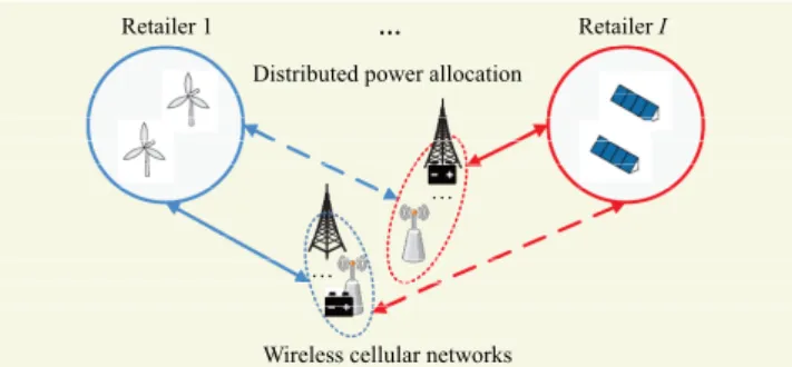
Owing to the intermittent power generation of renewable energy sources (RESs), future wireless cellular networks are required to reliably aggregate power from retailers. In this paper, we propose a distributed power allocation (DPA) scheme for base stations (BSs) powered by retailers with heterogeneous RESs in order to deal with the unreliable power supply (UPS) problem. The goal of the proposed DPA scheme is to maximize our well-defined utility, which consists of power satisfaction and unit power costs including added costs as a non-subscriber, based on linear and quadratic cost models. To determine the optimal amount of DPA, we apply dual decomposition, which separates the master problem into sub-problems. Optimal power allocation from each retailer can be obtained by iteratively coordinating between the BSs and retailers. Finally, through a mathematical analysis, we show that the proposed DPA can overcome the UPS for BSs powered from heterogeneous RESs.
Keywords: Base stations, Retailers, Heterogeneous renewable energy sources, Unreliable power supply, Distributed power allocation, Dual decomposition.
Manuscript received Nov. 18, 2015; revised Apr. 4, 2016; accepted May 24. 2016. This work was partly supported by Institute for Information & communications Technology Promotion (IITP) grant funded by the Korea government (MSIP) (B0101-16-1270, Research on Communication Technology using Bio-Inspired Algorithm) and (No.B0101-16-1365, Development of Technology for Integrated Energy Management Service of Building and Community and Their Energy Trading)
Seung Hyun Jeon ([email protected]) and Jun Kyun Choi ([email protected]) are with the School of Electrical Engineering, KAIST, Daejeon, Rep. of Korea.
Joohyung Lee (corresponding author, [email protected]) is with the Advanced Communication Laboratory, Samsung Electronics, Suwon, Rep. of Korea.
I. Introduction
With the explosion of small cells used to sustain mobile traffic growth for ubiquitous access, the operation expenditures caused by the power consumption over wireless cellular networks has severely increased, as reflected in our electric bills [1], [2]. For example, as the radio access part of wireless cellular networks, base stations (BSs) account for over 60% of the total energy cost [2], [3]. To reduce the power consumption at a BS, researches on energy-efficient BS operations such as switching off redundant BSs with low traffic [3]–[8] or traffic-load based dynamic BS operations [5], and minimizing the supplied power [9], have been carried out. Nevertheless, owing to the increasing infrastructure of information and communication technology (ICT), with approximately 2% for CO2 gas emissions [3], [7], wireless cellular providers will be forced to pay the additional pollutant emissions cost for protection of the global environment. Accordingly, as the power generation cost from renewable energy sources (RESs) has been decreasing, the main energy sources for BS operations have shifted from conventional energy sources to RESs as a way to reduce operation expenditures [1].
The use of RESs as the main power supply is considerably challenging because there is an unreliable power supply (UPS) problem caused by their intermittent generation [5], [8], [10], [11]. Nevertheless, continuing development in battery storage and utilizing aggregated energy sources from retailers can boost the sole use of RESs for BS operations without a conventional power supply [5], [8], [10]–[12]. In gencral, an RES can provide a constant power supply using battery storage
A Distributed Power Allocation Scheme for Base
Stations Powered by Retailers with Heterogeneous
Renewable Energy Sources
Fig. 1. Distributed power allocation scheme for a BS.
Retailer 1 … Retailer I
Distributed power allocation
…
…
Wireless cellular networks
to meet the power required by the BS and prevent an intermittent generation [13]. Moreover, the request for a power supply for a BS from retailers can be considered using a distributed power allocation (DPA) algorithm [5], [8]. Therefore, retailers with RESs are required to power the BSs.
To achieve a reliable power supply to BSs powered by RESs, Niyato proposed an adaptive power supply system associated with a single BS, where an RES, battery storage, and an adaptive power controller are considered [12]. Here, the battery storage of a BS is considered for reducing the variation in power; however, the BS still depends on a single power (SP) supply from the power grid. Regarding an SP by retailers, Bu and others proposed a Stackelberg-game based optimal energy procurement for BSs powered by retailers [5]. Ghazzai and others proposed the use of particle swarm optimization and genetic-algorithm based optimized energy procurement from retailers [8]. Both solutions find the DPA through utility-based cooperation between retailers and BSs, which is characterized by the different unit price and the pollutant levels of the energy sources used by retailers. However, the DPA in [5] and [8] does not take into consideration that RESs provide no CO2 emissions [14], and a wireless cellular provider having a contract with at least one retailer should exist. Thus, they should not be treated equally by each retailer. Moreover, according to a previous work [8], because the total aggregated power for the BSs is supplied sufficiently from the power grid with CO2 emissions, they cannot find the optimal DPA for a BS operation powered from pure RESs. Hence, in contrast with the previous work focusing on a reduction in the pollutant emissions for BSs, our goal is to find the optimal power allocation to maximize the utilization of heterogeneous RESs from retailers.
In this paper, we propose a DPA mechanism to solve the UPS problem for a BS, which can be insufficiently powered through the intermittent generation of an RES. Each retailer supplies power using different RESs, such as Photovoltaic (PV) panels and wind turbines [15]. To determine the costs for power supplied by retailers, two general cost models are considered: a linear energy cost model [16], [17] and a
quadratic energy cost model [16], [18]. Furthermore, to deal with the DPA under the UPS, our proposed BS operation scenarios consider the power generation capacity, different unit power costs for the RESs and non-subscribers, and variations in an insufficient power supply. Meanwhile, we assume that the BSs determine their required operational power considering the user traffic load and the portion of fixed operation power for a given period from the power consumption model for the BS operation used in [4], and BSs periodically request their required operational power to the retailers. In our work, we present an optimization problem to find the DPA based on cooperation between the BSs and retailers.
The contributions of this paper are summarized as follows: ▪ We deal with the UPS problem for BSs powered from RESs.
To cope with an insufficient power supply, we consider that each retailer gives a higher priority to providing power to its own subscribers (that is, BSs with a contract) than to non-subscribers (that is, BSs without a contract).
▪ We propose a DPA algorithm from the heterogeneous RESs of retailers. To find the optimal DPA by considering the BS operation scenarios, we utilize dual decomposition, which consists of sub-problems and a master problem. First, dual variables such as the price of the resources and coordination parameters are iteratively calculated though dynamical coordination between the BSs and retailers, and we can then obtain the optimal DPA from retailers through the low complexity time and iterations.
▪ Finally, based on experimental and public-data based analysis results, the proposed DPA can overcome the UPS for BSs powered from heterogeneous RESs.
The remainder of this paper is organized as follows. We briefly introduce the system model in Section II. The DPA problem formulation and algorithm are then presented in Section. III and IV, respectively. Section V shows the numerical results based on the experimental and public data, as well as a complexity analysis. Finally, Section VI provides some concluding remarks.
II. System Model
In this section, we address the DPA for BSs powered by heterogeneous RESs of retailers, as shown in Fig. 1. We define the arrival of mobile traffic according to a file transfer protocol traffic model, which is widely adopted in 3GPP [19]. There are M BSs denoted by set M = {1, 2, ... , m} in the geographical region, where a set of retailers I = {1, 2, ... , i} supply power from different RESs. We assume that file-transfer requests to BS m arrive with a user arrival rate λm and mean file size δm,
and hence the traffic load density is defined as ρm = λmδm < ∞
power control techniques adopted by the BS. Each BS, m M with maximum bandwidth capacity Cm, owned by a wireless
cellular provider is powered from its own home retailer (that is, the BSs with a contract), but can also procure power from other retailers as a non-subscriber. Suppose that each retailer uses different RES units (for example, PV panels and wind turbines). The power generation capacity of a RES owned by retailer i for the BSs can be expressed as gi.
The set of BSs that are powered by the RES of the retailer i is denoted as Mi M. The subset of BSs that are powered by
the energy source of home retailer i is denoted as Mi,1, and is Mi,2 otherwise. That is, Mi,1∪Mi,2 = Mi and Mi,1 ∩ Mi,2 = .
For classification, BS m Mi,1 is referred to as a subscriber of
retailer i, whereas BS m Mi,2 is referred to as a
non-subscriber of retailer i. Thus, a BS can access the available energy sources of retailers I simultaneously, and procure power from different energy sources at its location. Power allocation by an RES from retailer i to BS m is denoted as pm,i,
where m Mi,1 and i I. Let p be a power allocation vector
through the RESs of the retailers to the BSs, p = ( pm,i : m Mi), with pm,i = 0 if BS m is unavailable for the energy source
of retailer i.
III. Problem Formulation
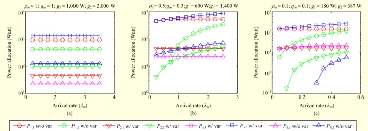
In this section, the problem of the power allocation for the BSs powered by the distributed RESs of the retailers is formulated. A distributed solution for such a problem is then proposed. For convenience, a detailed explanation of the notations used herein is provided in Table 1.
1. Power Consumption Model for Base Station Operation A power consumption model for a BS operation is generally proportional to its utilization [4], [20], [21]. Therefore, the operational power consumption required per BS m is derived as follows:
op fix fix
BS,m m, m 1 m m/ m m m m ,
P q q C P q P (1)
where qm [0, 1] represents the portion of fixed power
consumption to fix,
m
P which is the fixed operational power of BS m. The fixed operational power includes the power consumption for transmit antennas as well as the power amplifiers, feeder loss, cooling equipment, and signal processing [21]. If qm = 1, the BS can require the operational
power of BS m against the peak traffic. Otherwise, the BS can require operational power of BS m dependent upon the traffic load dynamically. In (1), ρm is the traffic load density to BS m,
and ρm/Cm is defined as the system load density. For example,
when the system load density is fully utilized, ρm/Cm = 1. In
Table 1. Notation for formulation.
Notation Explanation I Set of retailers
gi Power generation capacity of the RES of retailer i for BSs
Cm Maximum bandwidth capacity of BS m
ρm Traffic load density to BS m
pm,i Power allocation from retailer i to BS m
p Power allocation vector through RESs of retailers to BSs PBS, m Required constant power of BS m
min BS,m
P Minimum required power of BS m allowable for maximum variation (that is, power supply is insufficient)
max BS,m
P Maximum required power of BS m allowable for minimum variation (that is, max
BS,m
P is the same as PBS, m)
M Set of BSs in the geographical region M i Set of BSs powered by the RES of retailer i
M i,1 Set of subscribers among M i
M i,2 Set of non-subscribers among M i
M p1 Set of BSs without battery storage
M p2 Set of BSs with battery storage
common, each BS has various values (for example, a macro and micro BS) for a fixed operational power, as in [22], which is used for calculating the operational power required for BS
op BS,m
P . Using fixed operational power fix,
m
P the BS requires constant power PBS,m to the retailers. Because the retailers often cannot provide constant power to the BSs owing to an intermittent power generation, we assume that each BS has its own battery storage to handle the variation in power supply, as shown in Fig. 1 [10], [12]. The battery storage can be charged from the unused power during non-peak traffic [12].
On the other hand, considering a power supply allowable for such variation, we assume that the maximum and minimum operational power levels are required [12]. Thus, the BS requires the maximum power allowable for minimum variation
max BS,m
P and the minimum power allowable for maximum variation min
BS,m
P because the BSs are powered from their battery. We assume that max
BS,m
P is equal to PBS,m owing to almost no variation in the power generation. When all RESs in a geographical region reach their power capacity limitation, the power allocation with variation is degraded toward min
BS,m
P in order to support more power requests.
Thus, according to the choice of supply method for a constant power and the variation in power, the sets of BSs in the geographical region with and without battery storage are Mp2 and Mp1, respectively.
2. Utility Function A. Energy Cost Model
As an energy cost model for utility optimization [16], we consider two general cost models: a linear cost model1) [17] and a quadratic cost model2) [18]. Generally, a linear cost model has been applied for utility optimization [16], [17]. However, because each additional unit of power required to satisfy the increasing demand makes it more expensive to generate power to the consumer when considering the different power costs from heterogeneous RESs, the quadratic cost
model has also been considered as 2 1
2 1 0
( ) c c c
C q q q [18]. In this case, although the quadratic cost function captures the feature in which the marginal cost of generation is an increasing function of the output level, the quadratic cost model can abbreviate the linear and constant terms for simplicity [16], [18]. Therefore, the general cost function ci(pm,i) for the energy
source of retailer i to BS m is expressed as follows:
, 1) , 2 , , 2) , ( ) ( ) ) , . ( i m i i m i i m i i m i i m i c p c p c p c p c p (2)
In addition, the priority parameter οm,i assigned by the energy
source of retailer i to BS m is used to establish the differentiation in the power supply among other BSs without the home retailer, which is given by
,1 , ,2 , 1 , , , i m i i m M m M (3)
where α [0,1). Using the priority parameter, οm,i, retailers
place a higher cost on the energy sources for other BSs compared to their own subscribers. This is achieved by setting οm,i to charge an additional cost for using energy sources. B. Proposed Utility Function
Let um,i(pm,i) denote a utility function of retailer i allocating
power pm,i to BS m through an energy source. The utility
function is defined as
, , 1 , 2 , , ,1 ( ) ln(1 ) ( )(1 (1 ) , , m i m i m i i m i m i i u p p c p m M (4)where η1 and η2 are the weighting factors of the first and second terms, respectively. The utility function represents the satisfaction from the allocated power pm,i. The first term uses a
logarithmic utility function for the DPA because it is widely used in the literature for quantifying the satisfaction with diminishing returns [11], [23]. The second term represents the cost incurred by the BSs for allocated power. Based on the energy cost model in (2) with the priority parameter, retailers differentiate subscribers from non-subscribers for the charged
Proposition 1. The proposed utility um,i(pm,i) has a concave
function and a unique solution for the linear and quadratic energy cost model.
Proof. Taking the second derivative of um,i(pm,i) with respect to pm,i based on the linear energy cost model, we have
2 2 , , 1 2 2 , 1 , ( ) 0, 1 m i m i m i m i u p p p (5)where η1 is larger than zero. Taking the second derivative of um,i(pm,i) with respect to pm,i based on the quadratic energy cost
model, we also have
2 2 , , 1 2 1 , 2 2 , 1 , 1 (1 ) 0, 1 m i m i i m i m i m i u p c p p (6)where η2, ci, and 1 − om,i are larger than zero.
Therefore, the proposed utility um,i(pm,i) is a concave function
and a unique solution for pm,i. ■
power cost. As a result, each retailer places a higher priority on allocating its energy source to its subscribers as compared to the other BSs that are non-subscribers. According to the second term, we reflect the dissatisfaction with the penalty cost as a non-subscriber, which gives rise to increasing operation expenditures. There are two major motivations for designing this utility function. First, because the proposed utility is a concave function [24], from Proposition 1, it can guarantee the existence of a global optimal point.
Therefore, the objective of power allocation for the energy source of each retailer is to maximize the total utility, which is the sum of the power supplied from the energy source of retailer i for BS m, given by
, , ( ) ( ), , i i m i m i m M U u p i I
p (7) ( ). i i I U U
p (8) Next, we describe the following several constraints for the power allocation: power generation capacity, constant power supply, and power supply with variations. The allocated power from each retailer i with the energy source should be within the power generation capacity gi, given by, , . i m i i m M p g i I
(9) For a constant power, the total amount of power allocated from the available energy sources to the given BS m should satisfy the required power PBS,m,, BS, , 1. m i m p i I p P m M
(10)On the other hand, for variable power, the total amount of power allocated from the available energy sources to the given BS m should be within the range between the minimum required power allowable for the maximum variation min
BS,m
and the maximum required power allowable for the minimum variation max BS,m P , min max BS,m m i, BS,m, p2. i I P p P m M
(11)Thus, we formulate the following optimization problem [24], whose objective is to maximize the satisfaction of all BSs powered with constraints in terms of constant power, with variations in power, and the power generation capacity, as follows: 0 max ( ) s.t. (9) (11). i i I U
p p (12)Following the definition of the utility function in (4), (7), and (8), the objective function of problem (12) is concave by Proposition 1, and problem (12) has linear constraints. Therefore, the problem transformed into
0
min i IUi( )
p p
can become a convex optimization problem, which also creates the local and global maximums [24]. Because the constraints introduced in (10) and (11) are coupling constraints, it is difficult to obtain a distributed solution of (12) at each retailer. Thus, a distributed solution can be developed using the dual decomposition of (12) [25]. The constraint defined in (11) can be rewritten in the following forms:
max , BS, , 2, m i m p i I p P m M
(13) min , BS, , 2. m i m p i I p P m M
(14)The Lagrange dual function [24] for (12) using the constraints of (9), (10), (13), and (14) can be expressed as
1 2 2 1 2 , , BS, (1) max BS, , (2) min , BS, , , , , ( ) , i p p p i i i m i i I i I m M m m i m m M i I m m m i m M i I m m i m m M i I L U g p p P P p p P
p λ σ μ μ p (15) where λ = (λi : i I), σ = (σm : m Mp1), μ(1) = ( : m Mm(1) p2), and μ(2) = ( (2) m : m Mp2) are vectors of the Lagrange
multipliers corresponding to the capacity constraint of (9) with λi ≥ 0, and the required power constraints of (10), (13), and
(14) with (1)
m
, (2)
m
≥ 0, respectively. The dual function can be expressed as
1 2
1 2
0 , , , max , , , , , h L p λ σ μ μ p λ σ μ μ (16) and the dual problem corresponding to the primal problem of(12) is
1 2
1 2 , min, 0, h , , , . λ μ μ σ λ σ μ μ (17)Because the primal problem of (12) is a convex optimization problem, a strong duality exists [24]. The optimal values for the primal and dual problems are equal. As a result, it is appropriate to solve (12) through its dual problem of (17). The maximization problem of (16) can be simplified as
1 2 1 2 1 2 , , , 0 , , , max ( ) . i p p i i m i m m i m m m i i I m M m M m M h U p p p
p
λ σ μ μ p (18) Consequently, each retailer can solve its own utility maximization problem, which is expressed as
1 2 1 2 , , , 0 max ( ) . i p p i i m i m m i m m m i m M m M m M U p p p
p p (19) The optimum allocation p for fixed values of dual variables (λ, σ, μ(1), and μ(2)) can be calculated by each retailer with an energy source by applying the Karush-Kuhn-Tucker conditions [24] on (19), and we thus have
1 2
, , , ( ) 0. m i m i i m m m m i u p p (20)Using the utility function of (4) and (20), we can calculate the optimal power allocation *
,
m i
p using the linear and quadratic cost models. Therefore, the optimal solution can be described as
1 1 * , 2 {1, 2}, 4 , {3, 4 , }, 2 l l m i l l l l l A l A p B B A C l A (21)
where the notion [·]+ is a projection on the positive orthant to account for the fact that p ≥ 0. In (21), Al is a parameter with l =
{1, 2, 3, 4}, which is classified according to the energy cost model and the usage of battery storage through a variation in the power supply, with the exception that parameters Bl and Cl
with l include sets of {3, 4} as follows: • Linear cost model
1
1 2 , if 1 and 1 (1 ) , p i m i i m m M A c l (22)
2 1 2 2 2 1 , if 1 , d ) n 1 a ( p i m i i m m m M A c l (23) • Quadratic cost model
1 3 1 2 , 3 2 , 1 1 3 1 2 1 (1 ) , 2 if 3 and 1 (1 ) , , p i m i i m i i m i m m M B C l A c c (24)
2 4 1 2 , 1 2 4 2 , 1 1 2 4 1 2 1 (1 ) , 2 1 (1 ) ( ), ( ) f 4 and . i p i m i i m i i m m i m m m M A c c C l B (25)On the other hand, the optimum values of dual variables (λ, σ, μ(1), and μ(2)) for the given optimum allocation *
,
m i
p can be calculated by solving the dual problem of (17).
For a fixed allocation p, the dual problem of (17) can be simplified as 1 1 2 2 2 , 0 , BS, (1) max BS, , 0 (2) min , BS, 0 min min min min . i p p p i i m i i I m M m m i m m M i I m m m i m M i I m m i m m M i I g p p P P p p P
λ σ μ μ (26)For a differentiable dual function, a gradient descent method [24], [26] can be applied to calculate the optimum values for dual variables (λ, σ, μ(1), and μ(2)), given by
1
1 ,( ) , i i i i m i m M t t g p t
(27)
1
2 ,( ) BS, , m m m i m i I t t p t P
(28) 1
1
max
3 BS, , 1 , m m m m i i I t t P p t
(29) 2
2 min 4 , BS, 1 ( ) () , m m m i m i I t t p t P
(30)where t is the time index of the iteration and , with s = {1, 2, s
3, 4} being a sufficiently small fixed step size. Convergence toward the optimum solution is guaranteed because the gradient of (26) satisfies the Lipschitz continuity condition [26], [27]. Therefore, DPA pm,i of (21) converges to the optimum
solution, although BS m dynamically coordinates the heterogeneous RESs of the retailers.
Next, we consider simple BS operation scenarios for the
DPA between only two retailers and two BSs.
IV. Distributed Power Allocation Algorithm
The proposed decomposition method for the optimization problem of (12) has two levels [25], as depicted in Algorithm 1.
Algorithm 1. Distributed Power Allocation Algorithm
1: Parameters: each energy source needs its utility Ui (7), power
generation capacity, energy cost model (2), and required power demand of the BSs, which is determined by the traffic load and the portion of fixed power consumption (1).
2: Initialization: set t = 0 and dual variables (λ, σ, μ(1), and μ(2)) are defined as non-negative values except for σ.
3: Repeat the iteration.
(a) According to the energy cost model, the optimal power acquired from different energy sources of the retailers is locally calculated through (21) using the initial dual variables, and each retailer then allocates the optimal power.
(b) The retailers update their price for power to be supplied using the gradient descent method (27), and broadcast the new price
λi(t + 1) to the BSs.
(c) The BSs update their coordination parameters (28)–(30) using the gradient descent method and broadcast the coordination parameters to the retailers.
(d) Set t ← t + 1 and go to step (a) (until satisfying the termination criterion).
The first is a lower level where the sub-problems are solved at each retailer to find the optimum power allocation *
,
m i
p . The sub-problems defined in (19) have the optimum solution (21) based on parameters (22)–(25) considering the energy cost model and the use of battery storage through a variation in the power supply. In the case of the linear cost model, we can calculate the optimal solution based on (22) and (23). Similarly, in the case of the quadratic cost model, we can calculate the optimal solution based on (24) and (25).
The other is a higher level, where the master problem exists. The master problem is defined in (26), and the optimum solution is obtained through iterations for the dual variables defined in (27) through (30). Thus, the master problem is to set the dual variables (λ, σ, μ(1), and μ(2)) to coordinate the sub-problems at each retailer.
Following the classical interpretation of λi in economics as
the price of the resources [27], the price of the energy source of retailer i is given. Thus, it serves as an indication of the capacity limitation experienced by the energy source of retailer i. When the total power demand for the BSs from the energy source of retailer i reaches the limitation of the power generation capacity gi, the price λi for the supplied energy sources increases in order
to denote the expensive use of the energy sources. On the other hand, σm is a coordination parameter used for BSs powered
continuously without variation, whereas 1
m
and 2
m
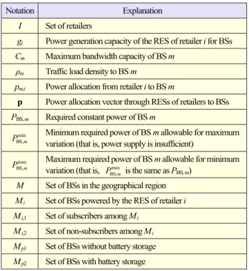
Fig. 2. Power allocation based on the linear energy cost model for BS operation scenarios: (a) mode 1, (b) mode 2, and (c) mode 3. 104 103 102 101 0 2 3 4 Arrival rate (m) Power allocation (W att) 103 102 101 100 0 1 2 3 Arrival rate (m) 103 102 101 100 10–1 0 0.2 0.4 0.6 Arrival rate (m) Power allocation (W att) Power allocation (W att) m = 1; qm = 1; g1 = 1,000 W; g2 = 2,000 W m = 0.5; qm = 0.3; g1 = 600 W; g2 = 1,400 W m = 0.1; qm = 0.1; g1 = 180 W; g2 = 387 W (a) (b) (c)
P1,1 w/o var P1,2 w/o var P2,1 w/ var P2,2 w/ var P3,1 w/ var P3,2 w/ var P4,1 w/o var P4,2 w/o var
the coordination parameters used for BSs with variations in power.
V. Numerical Results
This section presents analytical results and a complexity analysis for optimization problem (12) using Algorithm 1, based on experimental and public data.
1. Experimental Data Based Analysis
There are four BSs (M = 4) in a geographical region. BSs 1 and 2 are owned by wireless cellular provider 1 (C1), and BSs 3 and 4 are owned by wireless cellular provider 2 (C2). BSs 1 and 3 are macro BSs, and the other two are micro BSs. We assume that the operational power required for the macro and micro BSs is set as 1,350 and 144.6 W, respectively [22]. BS 2 of C1 and BS 3 of C2 have some battery storage to support a small amount of power owing to variations in the power supply. However, the battery capacity per BS is still limited to 2 kWh/h [12]. Two retailers can supply C1 and C2 within the given geographical region with power generated from PV panels and wind turbines, which are located onshore [28]. In particular, the power generation capacity of retailer 1 (R1) with wind turbines is insufficient against the required power for C1. On the contrary, retailer 2 (R2) with PV panels provides sufficient power to C2. To deal with the DPA under the UPS, we consider three BS operation scenarios: without regard to traffic load (mode 1), without using the battery storage of the BS but with a dependence on the traffic load (mode 2), and using the battery storage of the BS but with dependence on the traffic load (mode 3). Here, modes 1 and 2 indicate that the total aggregated power generation of all retailers is sufficient to supply power into C1 and C2, whereas mode 3 indicates that the total aggregated power generation of all retailers is
insufficient owing to the weather conditions. We assume that the unit power cost ci is set as 60 USD/MWh for c1 and 280 USD/MWh for c2 [28]. The unit power cost ci is
determined based on the levelized cost of electricity (LCOE), which is the average cost of an RES considering the installation cost. In addition, qm for each BS is dependent on the amount of
power supplied from retailers or traffic load as the user arrival rate (λm), which is classified as peak (100%), moderate (50%),
or low (10%). Other system parameters are set as follows: Cm
is 20 Mbps, om,i = 0.4, δm is 500 kbytes, and η1 = η2 = 1.7045.
Figure 2 shows the power allocation against traffic load based on the linear energy cost model. Figure 2(a) presents the power allocation against the peak traffic as mode 1. Thus, power supplied from each retailer is allocated completely without regard to the traffic load (that is, qm = 1.). Owing to the
lack of power generation from R1, R2 provides the remaining power to BSs 1 and 2 of C1. Although BSs 2 and 3 have battery storage with a variation in power supply, they do not need to use this solution owing to sufficient power generation from the retailers. Here, BSs 1 and 4 are supplied with constant power without variation in the power supply. Thus, all micro and macro BSs can assign the maximum operation power as 144.6 W and 1,350 W, respectively.
Figure 2(b) shows the power allocation against moderate traffic as mode 2. We assume that qm = 0.3 dependent on a
somewhat small power generation. BSs 1 and 2 are powered by R2 after the arrival rate reaches 0.5. Similar to Fig. 2(a), although the power required is reduced owing to a moderate traffic level and decrease in qm, there is no difference in power
allocation for BSs 2 and 3 caused by a variation in the power supplied from the retailers owing to the sufficient power generation within the given geographical region. Thus, all micro and macro BSs can sufficiently assign the required operation power of 93.99 W and 877.5 W, respectively.
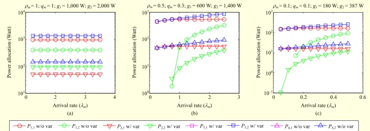
Fig. 3. Power allocation based on the quadratic energy cost model for BS operation scenarios: (a) mode 1, (b) mode 2, and (c) mode 3.
104 103 102 101 0 2 3 4 Arrival rate (m) Power allocation (W att) 103 102 101 100 0 1 2 3 Arrival rate (m) 103 102 101 100 10–1 0 0.2 0.4 0.6 Arrival rate (m) Power allocation (W att) Power allocation (W att) m = 1; qm = 1; g1 = 1,000 W; g2 = 2,000 W m= 0.5;qm = 0.3;g1 = 600 W;g2 = 1,400 W m = 0.1; qm = 0.1; g1 = 180 W; g2 = 387 W (a) (b) (c)
P1,1 w/o var P1,2 w/o var P2,1 w/ var P2,2 w/ var P3,1 w/ var P3,2 w/ var P4,1 w/o var P4,2 w/o var
Figure 2(c) shows the power allocation against low traffic as mode 3. We assume qm = 0.1 dependent on a small power
generation. BS 2 is powered by R2 after the arrival rate reaches 0.05. On the other hand, BS 1 is powered by R2 after the arrival rate reaches 0.1. We assume that BSs 2 and 3, which are allowed a variation in power, can be powered within 0.5 W of their battery capacity. Unlike in Figs. 2(a) and 2(b), BSs 2 and 3 use their own battery storage at approximately 0.5 W and 0.45 W, respectively.
Therefore, BSs of C1 are supported from R2 as non-subscribers, and C1 can then solve the UPS caused by the three BS operation scenarios.
Figure 3 shows the power allocation for the traffic load based on the quadratic energy cost model. Figure 3(a) presents the power allocation against the peak traffic as mode 1. Power supplied from each retailer is allocated completely without regard to the traffic load, as shown in Fig. 2(a). Contrary to Fig. 2(a), BS 4 is powered by R1 with insufficient power generation. Because the power allocation for BSs 1 and 2 from R2 based on the quadratic cost model is larger than that based on the linear cost model, BS 4 is powered inversely by R1 owing to the lack of an SP from R2. Thus, a multiple power (MP) supply can exist under a lack of power generation among retailers. Furthermore, BSs 2 and 3 do not consider any variations in power supply owing to a sufficient power generation from R2, as shown in Fig. 2(a).
Figure 3(b) shows the power allocation against moderate traffic as mode 2. BS 2 is powered by R2 after the arrival rate reaches 0.25. On the other hand, BS 1 is powered by R2 after the arrival rate reaches 0.5. As shown in Fig. 2(b), BSs 2 and 3 do not suffer from a variation in power supplied from retailers owing to the procuring of sufficient power for the total power generation. However, for the same reason provided for Fig. 2(a), BSs 1 and 2 of C1 and BS 4 of C2 are powered by
R1 and R2, respectively. Here, as a subscriber, power allocation for BS 4 from R2 is larger than that for BS 2 from R1 after the arrival rate reaches 1.25. Furthermore, as a non-subscriber, power allocation for BS 2 from R2 is larger than that for BS 4 from R1 after the arrival rate reaches 1.
Figure 3(c) shows the power allocation against low traffic as mode 3. BSs 1 and 2 are powered by R2 after the arrival rate reaches 0.05 and 0.1, respectively. Differing from Figs. 3(a) and 3(b), BSs 2 and 3 use their own battery storage at approximately 0.5 and 0.45 W, respectively. Compared with Fig. 2(c), an MP supply is allocated from R1 and R2. However, BS 4 as a non-subscriber is first powered by R1. Next, after the arrival rate reaches 0.3, BS 4 as a subscriber is powered by R2. Moreover, power allocation for BS 4 from R1 is larger than that from R2. The reason for providing a large amount of power to non-subscribers is because, although additional unit power cost for BS 4 as a non-subscriber is charged, the unit power cost of R1 is still cheaper than that of R2.
Therefore, the BSs of C1 are supported from R2 as non-subscribers, and BS 4 of C2 is also supported from R1 as a non-subscriber. Furthermore, C1 and C2 can solve the UPS caused by three BS operation scenarios. We finally show the total utility for only the quadratic energy cost model.
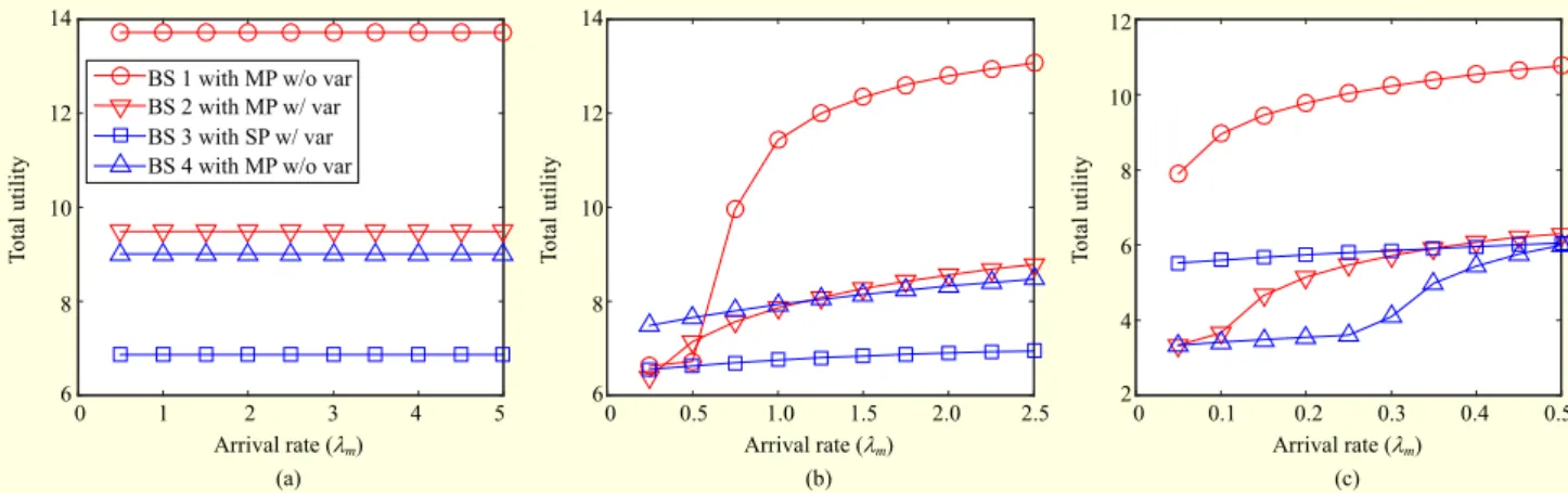
Figure 4 shows the total utility based on the quadratic cost model. Figure 4(a) shows the total utility against peak traffic as mode 1. As mentioned in relation to Fig. 3(a), BSs 1, 2, and 4 are powered by an MP supply by the retailers. On the contrary, BS 3 is powered by an SP from R2. Although BSs 2 and 3 are powered by an MP supply, BS 2 has a higher level of satisfaction than BS 4 because the power supplied from R2 for BS 2 is larger than that from R1 for BS 4, as shown in Fig. 3(a).
That is, BS 2 uses more MP supply than BS 4. In addition, BS 3 has the worst satisfaction rate owing to the expensive unit power cost and power allocation by the SP.
Fig. 4. Total utility based on the quadratic energy cost model for BS operation scenarios: (a) mode 1, (b) mode 2, and (c) mode 3. 14 12 10 8 6 0 1 2 3 4 5 Arrival rate (m) To tal utility (a) 14 12 10 8 6 0 0.5 1.0 1.5 2.0 2.5 Arrival rate (m) To tal utility (b) 12 10 8 4 2 0 0.1 0.2 0.3 0.4 0.5 Arrival rate (m) To tal utility (c) 6
BS 1 with MP w/o var BS 2 with MP w/ var BS 3 with SP w/ var BS 4 with MP w/o var
Figure 4(b) presents the total utility against moderate traffic as mode 2. Because BS 1 is powered from R2 after the arrival rate reaches 0.5, as shown in Fig. 3(b), satisfaction regarding BS 1 skyrockets. In particular, because power supplied from R2 for BS 2 is larger than that from R1 for BS 4 after the arrival rate reaches 1, as shown in Fig. 3(b), BS 2 has a higher level of satisfaction than BS 4. Moreover, satisfaction regarding BS 3 increases slightly owing to a reflection in the quadratic energy cost model by the increased power allocation, as shown in Fig. 3(b). Figure 4(c) presents the total utility against low traffic as mode 3. Because BS 4 is powered from R2 after the arrival rate reaches 0.3, as shown in Fig. 3(c), satisfaction regarding BS 4 also increases. However, satisfaction regarding BS 4 is still less than that of BS 2 because power supplied by R1 as a non-subscriber is larger than that by R2 as a non-subscriber, as shown in Fig. 3(c). Therefore, satisfaction regarding our utility is more dependent on the amount of power supplied from the home retailer than from other retailers.
Therefore, our proposed utility allocates MP supply to the BSs under the quadratic cost model. With sufficient power generation in the given geographical region, the proposed utility allocates a large amount of power from other retailers. Meanwhile, with insufficient power generation in the given geographical region, the proposed utility allocates considerable power from the home retailer. Moreover, wireless cellular providers should make a contract with a retailer as a home retailer to supply power from the RESs at a low unit power cost under the quadratic energy cost model.
2. Public Data Based Analysis
This subsection presents a public mobile traffic based analysis, as shown in Fig. 5, which shows the load density for mobile download traffic in London. We then classify the system load density as follows: peak (0.6 ≤ ρ ≤ 1), moderate (0.3 ≤ ρ < 0.6), and low (0 ≤ ρ < 0.3). First, we
Fig. 5. Load density for mobile data downloaded in London [29].
Peak Moderate Low
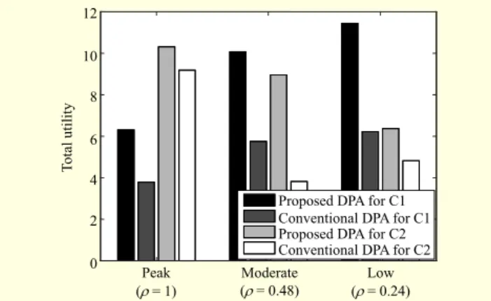
consider that cellular networks can account for a maximum of 0.0054% available power from the generation capacity of each retailer according to the electricity generation for the ICT [30], CO2 emission, of mobile systems [31], and power consumption of the BSs [2], [3]. This is a reasonable assumption because the retailer meets the total energy demand within the regions. Thus, considering the weather conditions, the generation capacity of the retailers is set as follows: wind turbines, from 4,320 W to 1,296 W; and solar panels, from 1,620 W to 2,268 W. The LCOE for onshore wind turbines and solar panels are set as 53 USD/MWH and 113 USD/MWh, respectively [28]. In addition, deviating from the experimental results, we extend the numbers of BSs to 8, where each cellular provider owns two macro and two micro BSs. Here, half of each type of BS has its own battery storage. Next, we compare the proposed and traditional DPAs in Fig. 6 [8], which considers the BS operation scenarios and parameters based on the quadratic energy cost model as follows: mode 1 for peak, mode 2 for low, and mode 3 for moderate levels, and the battery capacity of the BS supports only 1 day, and qm is assigned as 1, 0.5, and 0.25,
respectively. In Fig. 6, satisfaction of the proposed DPA is improved over the traditional DPA because the traditional scheme uses all of its own battery capacity available for reducing the CO2 emissions, and maximizing the MP can improve the satisfaction regarding the power allocation.
Fig. 6. Comparison between the proposed and conventional DPAs. Peak (= 1) 12 10 8 6 4 2 0 Moderate (= 0.48) Low (= 0.24) To tal utility
Proposed DPA for C1 Conventional DPA for C1 Proposed DPA for C2 Conventional DPA for C2
3. Complexity Analysis
The time complexity of the proposed DPA algorithm is calculated as Θ(nmi), where n, m, and i are the number of iterations, BSs, and retailers, respectively. The numerical results indicate that the number of iterations required to find the optimal DPA reaches three for the three BS operation scenarios. Using the tic-toc function of MATLAB, the computation times for both DPA schemes in Fig. 6 are similar, within about 0.05 s. However, this time is proportional to the amount of DPA. All tests were conducted on a laptop featuring an Intel Core i7-5500U CPU and running Windows 10 Home version. The clock of the machine was set to 2.40 GHz with 8 GB of memory. Although the number of BSs increased by two-fold, the computation time does not differ much. However, owing to the power distribution loss [11] and intermittent power generation capacity of the retailers, a single retailer cannot support a power supply to many BSs. Thus, we consider the additional computation time for the DPA to not be serious.
VI. Conclusion
This paper dealt with the unreliable power supply (UPS) problem for an insufficient BS power supply. We presented a distributed power allocation (DPA) scheme from the heterogeneous RESs of retailers, such as PV panels and wind turbines, when considering the traffic load, power generation capacity, different unit power costs for the RESs and non-subscribers, and variations in an insufficient power supply. Using the dual decomposition, the proposed algorithm procures optimal power allocation from each retailer through a dynamic coordination between the BSs and retailers in an iterative manner. The analytical results show that the proposed DPA maximizes the utilization of the distributed RESs, and that the uncertainty regarding the reliable power supply from heterogeneous RESs to the BSs can be reduced.
References
[1] J.G. Andrews et al., “What Will 5G Be?” IEEE J. Sel. Areas
Commun., vol. 32, no. 6, June 2014, pp. 1065–1082.
[2] Y. Chen et al., “Fundamental Trade-offs on Green Wireless Networks,” IEEE Commun. Mag., vol. 49, no. 6, 2011, pp. 30–37. [3] E. Oh et al., “Toward Dynamic Energy-Efficient Operation of Cellular Network Infrastructure,” IEEE Commun. Mag., vol. 49, no. 6, June 2011, pp. 56–61.
[4] K. Son et al., “Base Station Operation and User Association Mechanisms for Energy-Delay Tradeoffs in Green Cellular Networks,” IEEE J. Sel. Areas Commun., vol. 29, no. 8, Sept. 2011, pp. 1525–1536.
[5] S. Bu et al., “When the Smart Grid Meets Energy-Efficient Communications: Green Wireless Cellular Networks Powered by the Smart Grid,” IEEE Trans. Wireless Commun., vol. 11, no. 8, Aug. 2012, pp. 3014–3024.
[6] K. Son and B. Krishnamachari, “SpeedBalance: Speed-Scaling-Aware Optimal Load Balancing for Green Cellular Networks,”
IEEE Proc. INFOCOM, Orlando, FL, USA, Mar. 25–30, 2012,
pp. 2816–2820.
[7] Y.S. Soh et al., “Energy Efficient Heterogeneous Cellular Networks,” IEEE J. Sel. Areas Commun., vol. 31, no. 5, May 2013, pp. 840–850.
[8] H. Ghazzai et al., “Optimized Smart Grid Energy Procurement for LTE Networks Using Evolutionary Algorithms,” IEEE Trans.
Veh. Technol., vol. 63, no. 9, Nov. 2014, pp. 4508–4519.
[9] H. Holtkamp et al., “Minimizing Base Station Power Consumption,” IEEE J. Sel. Areas Commun., vol. 32, no. 2, Feb. 2014, pp. 297–306.
[10] D. Li et al., “Decentralized Energy Allocation for Wireless Networks With Renewable Energy Powered Base Stations,”
IEEE Trans. Commun., vol. 63, no. 6, June 2015, pp. 2126–2142.
[11] J. Lee et al., “Distributed Energy Trading in Microgrids: A Game-Theoretic Model and Its Equilibrium Analysis,” IEEE Trans. Ind.
Electron., vol. 62, no. 6, June 2015, pp. 3254–3533.
[12] D. Niyato, X. Lu, and P. Wang, “Adaptive Power Management for Wireless Base Station in a Smart Grid Environment,” IEEE
Wireless Commun. Mag., vol. 19, no. 6, 2012, pp. 1536–1284.
[13] J.M. Carrasco et al., “Power-Electronic Systems for the Grid Integration of Renewable Energy Sources: A Survey,” IEEE
Trans. Ind. Electron., vol. 53, no. 4, June 2006, pp. 1002–1016.
[14] R.E.H. Sims, H.-H. Rogner, and K. Gregory, “Carbon Emission and Mitigation Cost Comparisons between Fossil Fuel, Nuclear and Renewable Energy Resources for Electricity Generation,”
Energy Poicy, vol. 31, no. 13, Oct. 2003, pp. 1315–1326.
[15] M. Patterson, N.F. Macia, and A.M. Kannan, “Hybrid Microgrid Model Based on Solar Photovoltaic Battery Fuel Cell System for Intermittent Load Applications,” IEEE Trans. Energy Convers., vol. 30, no. 1, Mar. 2015, pp. 359–366.
[16] A. Mohsenian-Rad et al., “Autonomous Demand-Side Management Based on Game-Theoretic Energy Consumption Scheduling for the Future Smart Grid,” IEEE Trans. Smart Grid, vol. 1, no. 3, Dec. 2010, pp. 320–331.
[17] S. Bu, F.R. Yu, and P.X. Liu, “A Game-Theoretical Decision-Making Scheme for Electricity Retailers in the Smart Grid with Demand-Side Management,” IEEE Int. Conf. Smart Grid
Commun., Brussels, Belgium, Oct. 17–20, 2011, pp. 387–391.
[18] P. Luh, Y. Ho, and R. Muralidharan, “Load Adaptive Pricing: An Emerging Tool for Electric Utilities,” IEEE Trans. Autom.
Control, vol. 27, no. 2, Apr. 1982, pp. 320–329.
[19] 3GPP TR 36.814, Further advancements for E-UTRA physical layer aspects (Release 9), Mar. 2010.
[20] F. Richter, A.J. Fehske, and G.P. Fettweis, “Energy Efficiency Aspects of Base Station Deployment Strategies for Cellular Networks,” IEEE Veh. Technol. Conf. Fall, Anchorage, AK, USA, Sept. 20–23, 2009, pp. 1–5.
[21] ITU-T Rec. Y.3022, Measuring energy in networks, Aug. 2014. [22] G. Auer et al., “How Much Energy is Needed to Run a Wireless
Network?” IEEE Wireless Commun. Mag., vol. 18, no. 5, Oct. 2011, pp. 40–49.
[23] S. Park et al., “Contribution-Based Energy-Trading Mechanism in Micro-Grids for Future Smart Grid: A Game Theoretic Approach,” IEEE Trans. Ind. Electron., vol. 63, no. 7, Jan. 2016, pp. 4255–4265.
[24] S. Boyd and L. Vandenberghe, Convex Optimization, Cambridge, UK: Cambridge University Press, 2004, pp.1–287.
[25] D.P. Palomar and M. Chiang, “A Tutorial on Decomposition Methods for Network Utility Maximization,” IEEE J. Sel. Areas
Commun., vol. 24, no. 8, Aug. 2006, pp. 1439–1451.
[26] D.P. Bertsekas, Nonlinear Programming, 2nd edition, Belmont, MA, USA: Athena Scientific, 2003, pp. 22–84.
[27] M. Ismail and W. Zhuang, “A Distributed Multi-Service Resource Allocation Algorithm in Heterogeneous Wireless Access Medium,” IEEE J. Sel. Areas Commun., vol. 30, no. 2, Feb. 2012, pp. 425–432.
[28] National Renewable Energy Laboratory (NREL), Levelized Cost
of Energy, Open Energy Information (OpenEI), 2011. Accessed
Nov. 9, 2015. http://en.openei.org/apps/TCDB/
[29] S. Grauwin et al., “Towards a Comparative Science of Cities: Using Mobile Traffic Records in New York, London, and Hong Kong,” Comput. Approaches Urban Environments, vol. 13, 2014, pp. 363–387.
[30] M.P. Mills, The Cloud Begins With Goal, Digital Power Group, 2011. Accessed Aug., 2013. http://www.tech-pundit.com/wp-content/uploads/2013/07/Cloud_Begins_With_Coal.pdf?c761ac [31] S. Zeadally, S.U. Khan, and N. Chilamkurti, “Energy-Efficient
Networking: Past, Present, And Future,” J. Supercomputing, vol. 62, no. 3, May 2011, pp. 1093–1118.
Seung Hyun Jeon received his BS degree in
computer science from Pukyung National University, Busan, Rep. of Korea, in 1999, and his MS degree from Korea Advanced Institute of Science and Technology (KAIST), Daejeon, Rep. of Korea, in 2009. He is currently a PhD candidate at KAIST. From 2010 to 2011, he worked as a research engineer at ETRI, Daejeon, Rep. of Korea. He was an editor of the International Telecommunication Union Telecommunication Standardization Sector for Recommendation Y.3022. He received a Best Paper Award at the International Conference on ICT Convergence in 2012. Currently, his main research interests include resource allocation and optimization, with a focus on bio-inspired communications and energy-efficient solutions for 5G networks and smart grids.
Joohyung Lee received his BS, MS and his PhD
degrees in the Department of Electronics Engineering at KAIST Daejeon, Rep. of Korea in 2008, 2010, and 2014, respectively. He was with the Department of Electronics Engineering, City University of, Hong Kong, as a visiting researcher from 2012 to 2013. In 2014, he joined Samsung Electronics, Suwon, Rep. of Korea, as a senior engineer. He Lee was a member of the GreenTouch Consortium. From 2010 to 2013, he contributed several articles to ITU-T SG 13. He received a Best Paper Award at the Integrated Communications, Navigation, and Surveillance Conference in 2011. His research interests include resource allocation and optimization, with a focus on resource management for 5G networks, green networks, smart grids, and network economics.
Jun Kyun Choi received his BS degree in
electronics from Seoul National University, Rep. of Korea, in 1982, and his MS and PhD degrees in electronics engineering from KAIST, Daejeon, Rep. of Korea, in 1985 and 1988, respectively. From June 1986 to December 1997, he was with ETRI, Daejeon, Rep. of Korea. In January 1998, he joined the Information and Communications University (presently, KAIST) as a professor. Since 1993, he has contributed to ITU-T recommendations as an editor, rapporteur, and head of the Korea delegation for ITU-T SG 13 on the ATM, MPLS (Y.1281), NGN (Y.2002, Y.2054), IPTV, and energy saving networks (Y.3022). He is an executive member of the Institute of Electronics Engineers of Korea, Seoul, Rep. of Korea, an editor board member of the Korea Information Processing Society, Seoul, Rep. of Korea, and a lifetime member of the Korea Institute of Communication Science, Seoul, Rep. of Korea. His main research interests include trusted information infrastructures, smart media platforms, and energy-saving solutions for the Internet of Things (IoTs) and smart grids.