Hysteresis and Averaging the Forecasts of Exchange Rates

(1)

of Exchange Rates

1

**Byeongseon Seo * and Jinho Kim**

Real exchange rates evolve independently of money supply shocks in accordance with long-run monetary neutrality. However, the prolonged disequilibrium errors of the Korean won―US dollar real exchange rates in the 1990s prior to the Asian financial crisis and the hike subsequent to the crisis indicate hysteresis of the real exchange rates. The hysteresis may originate from two sources, namely, the instability of the equilibrium relationship and the regime-dependent persistence of real exchange rates. The current paper provides a statistical evaluation of the hysteresis in the won^―dollar real exchange rates using forecast combination. The behavior of asymmetric mean reversion and regime-dependent persistence dominates the parameter instability in real exchange rates. A substantial improvement in predictive accuracy is observed as the forecasting model in- corporates the hysteresis effect.

Keywords: Forecast combination, Hysteresis, Instability, Persistence

JEL Classification: C53, F31, F37, G17

* Corresponding Author, Professor, Department of Food and Resource Economics, Korea University, Anam-Dong, Seongbuk-Ku, Seoul 136-701, Korea, (Tel) +82-2-3290-3032, (Fax) +82-2-953-0737, (E-mail) [email protected];

Graduate Student, Department of Food and Resource Economics, Korea Uni- versity, Anam-Dong, Seongbuk-Ku, Seoul 136-701, Korea, (Tel) +82-2-958-4088, (E-mail) [email protected], respectively. The authors thank M. Fukushige, H. Pyo, K. Shin, C. Song, and the participants at the annual conference of Japan Society of International Economics for their invaluable comments and suggestions. Special thanks go to the anonymous referees and the Editor for the useful comments and suggestions. This work was supported by the National Research Foundation of Korea Grant funded by the Korean Government (NRF- 2010-330-B00060).

[Seoul Journal of Economics 2011, Vol. 24, No. 3]

(2)

I. Introduction

The principle of long-run monetary neutrality implies that real exchange rates evolve independently of nominal shocks. However, recent movements in Korean won—US dollar real exchange rates reflect broad and persistent deviations from the equilibrium level based on the fundamental economic variables. This hysteresis may originate from the permanent change in the long-run relationship or from the regime- dependent persistence of real exchange rates. The current paper aims to provide a statistical assessment of the hysteresis using forecast combination. The instability of the long-run relationship and the asymmetric mean reversion behavior is analyzed.

The hysteresis in the Korean won—US dollar real exchange rate may be triggered by an exogenous shock, such as the Asian currency crisis, which can be regarded as a structural break. Hence, before and after the Asian crisis, the Korean economy may have experienced two different monetary regimes with significantly different interest rate levels (i.e., high before the crisis and low after the crisis). This may then change the nature of both the long-run and short-run relationship between nominal exchange rate and its fundamental determinants. Thus, iden- tifying the nature of the hysteresis in the real exchange rate is neces- sary, whether the hysteresis is the outcome of the permanent structural change or of the regime-dependent persistence.

Exchange rate forecasting models using real exchange rate information have been developed based on the price approach and the monetary approach. The price approach implies that the change in exchange rates is related to the differentials in domestic and foreign price levels.

However, the volatility of exchange rates is too high to be explained by sluggish price movement. Dornbusch (1976) devises a disequilibrium model showing that exchange rates respond excessively to unanticipated money supply shocks by assuming price rigidity. The idea of hysteresis was formalized by Dixit (1989) and Baldwin and Lyons (1994) as a means to link national competiveness and current accounts to the persistence of disequilibrium in real exchange rates. Contrary to long-run monetary neutrality, the notion of real exchange rate hysteresis asserts that nominal shocks may induce changes in real exchange rates in the long run.

The monetary approach, which was elucidated previously by Frenkel (1976), Mussa (1976), and Bilson (1978), is based on the international Fisher effect, in which the interest rate differentials are consistent with

(3)

the anticipated changes in the exchange rates. If the money supply is fixed, increases in the domestic interest rate raise the opportunity cost of holding currency, which lowers the demand for domestic currency and results in the depreciation of the exchange rates. Lucas (1982) devises an equilibrium model in which the equilibrium exchange rates are determined by the equilibrium conditions of goods and currency markets. The equilibrium level of the exchange rate is associated with the money supply and income in domestic and foreign countries. The equilibrium model is related closely to the monetary approach in that the exchange rate is determined by money and income. Moreover, the equilibrium model accompanies the functioning of the terms of trade, as well as the money supply and income.

In the current study, we evaluate the stability of the long-run relationship and the path-dependent persistence with asymmetric adjustments in the Korean won—US dollar exchange rates. The long-run relationships determined by the purchasing power parity and the equilibrium model are found to be stable. However, the adjustment of the exchange rates to the disequilibrium errors reveals asymmetry. Thus, the evidence of parameter instability in the won—dollar exchange rates is not significant, whereas the asymmetric adjustment is reflective of regime-dependent persistence.

The results of asymmetric mean-reversion behavior have been docu- mented in a variety of previous studies, such as those of Michael, Nobay, and Peel (1997), Obstfeld and Taylor (1997), and Taylor, Peel, and Sarno (2001). Most notably, Michael, Nobay, and Peel (1997) reveal a nonlinear adjustment of the US dollar real exchange rates using the smooth transition autoregressive model. Moreover, nonlinearity in nominal exchange rates has been evaluated in several previous studies. Engle and Hamilton (1990) and Engle (1994) apply the Markov regime-switching model.

Diebold and Nason (1990), Meese and Rose (1991), and Mizrach (1992) employ different non-parametric procedures. In the current paper, the asymmetric mean-reverting behavior in the Korean won—US dollar exchange rate is analyzed using the threshold vector error correction model (VECM) first developed by Hansen and Seo (2002).

The recent volatile movement in exchange rates entails increased risk and loss of welfare. The current study originates from medium-term and long-term predictions of the won—dollar exchange rates. The forecasting of exchange rates is currently both important and useful because the global financial crisis has seriously affected the relevant economic variables.

(4)

The unpredictability of exchange rates has a long history in the economic literature. According to the efficient market hypothesis, the exchange rate reflects all the information within the market, as shown previously by Meese and Singleton (1982). Meese and Rogoff (1983) first advance the exogeneity proposition, that is, that future changes in exchange rates are unpredictable using any economic variable. This unpredictability has been empirically assessed in several studies. For in- stance, Mark (1995) evaluates the information contents of the purchasing power parity and determines that the long-run equilibrium relationship provides some useful information for the forecasting of long-run exchange rates. In the current study, we evaluate the information on the long-run relationship inherent in the purchasing power parity and the equilibrium model.

The remainder of this paper is organized as follows. Section 2 provides a brief review of some theoretical models of foreign exchange rates.

Section 3 presents the econometric methods, and Section 4 provides the main results of the empirical analysis.

II. Theoretical Background

The forecasting model of exchange rates can be formulated based on the economic theory of exchange rate determination. First, the price approach is predicated on the purchasing power parity (PPP), which holds that the value of a currency in the domestic market is the same as that in the foreign market. Thus,

= ^*

P EP (1) where E is the nominal exchange rate, P the domestic price level, and P^* the price level in a given foreign country.

If the domestic price level rises, the currency value in the domestic country decreases, and the nominal exchange rate depreciates. The real exchange rate, R, is defined as the ratio of the value of a currency in the foreign country to the domestic value.

= EP*

R P (2) The PPP principle implies the stationarity of the real exchange rates.

Thus, it specifies the long-run equilibrium relationship as follows:

(5)

β β

= + 1 + 2 ^*

t t t t

w e p p (3)

where et is the nominal exchange rate, pt the domestic price level, and p^*t is the foreign price level in logarithms.

The price approach assumes that price changes are flexible, such that changes in the exchange rates reflect the inflation differentials between the two countries. However, the volatility of the exchange rates is too high to emerge strictly as a result of price movements. This stylized fact is frequently associated with Dornbusch’s overshooting hypothesis (1976), which states that goods prices are sticky and that exchange rates reflect all the short-run adjustments of the economy in response to unanticipated money supply shocks.

The notion of hysteresis was formally treated in the theoretical model of Dixit (1989) and Baldwin and Lyons (1994). The entry of a firm involves investment cost, and the exit entails the sunk costs associated with initial investment. Thus, there exists a band of inaction, in which neither the entry nor the exit can be determined. If an economy lies within this range, the competiveness or net foreign wealth can be affected. Thus, unanticipated money supply shocks can lead to real exchange rate hysteresis.

The volatility of the Korean won—US dollar exchange rates became high and pronounced during the financial crises of 1997 and 2008.

According to the hysteresis effect of real exchange rates, unanticipated monetary shocks influence real exchange rates in the long-run and short-run. Thus, the long-run relationship of determining the exchange rates may involve instability. The conventional models of forecasting the exchange rates assume the stability of the long-run relationship. Hence, evaluating the stability and incorporating the hysteresis effect are ne- cessary when attempting to forecast the exchange rates.

Second, the monetary approach specifies the exchange rates to be determined based on the demand and supply of domestic and foreign currencies. The increase in the supply of domestic currency lowers the value of the domestic currency, thus resulting in depreciation. The increase in income is associated with the increase in demand for domestic currency, subsequently improving the value of the domestic currency.

In the equilibrium (EQ) model elucidated by Stockman (1980) and Lucas (1982), exchange rates are determined by the equilibrium between the conditions of goods and money markets. Thus, the determinants of long-run exchange rate fluctuations in domestic and foreign countries

(6)

are money and income. Equilibrium exchange rates are associated with the money supply and income in domestic and foreign countries. The EQ model is closely related to the monetary approach, as explained by Frenkel (1976) and Mussa (1976), in which the exchange rate is determined by money and income. The EQ model accompanies the functioning of the terms of trade as well as the money supply and income.

The terms of trade are equivalent to the real exchange rate in equilibrium:

= ^*/ ^*

/ W EM Y

M Y (4)

where M(M^*) is the supply of domestic (foreign) currency, Y(Y^*) is the domestic (foreign) income, and W is the terms of trade between the home and foreign countries.

If we assume the stationarity of the terms of trade, an increase in the domestic money supply will result in a rise in the nominal exchange rate. The increase in domestic income reduces the nominal exchange rates. The terms of trade can be influenced by the preference bias for domestic or foreign goods. However, the preference bias is unlikely to persist; thus, the terms of trade are stationary.

The EQ model implies the stationarity of the terms of trade, spe- cifying the long-run equilibrium relationship as follows:

β β β β

= + 1 + 2 ^*+ 3 + 4 ^*

t t t t t t

w e m m y y (5)

where et denotes the nominal exchange rates, mt(m^*t) domestic (foreign) money stock, and y_t(y^*_t) the domestic (foreign) income in logarithms.

III. Econometric Methods

The forecast combination occupies a solid space in the econometric literature. Forecast averaging lowers forecast errors and improves the accuracy of predictions. In the current paper, we employ the forecast combination to isolate the relative contribution of the permanent parameter changes in the long-run relationship and the regime-dependent persistence of the disequilibrium errors in explaining the hysteresis in real exchange rates.

(7)

The parametric instability in the long-run relationship ushers in permanent changes in the parameters at the break point, t^*.

β

= 1^'

t t

w x for t≤t^*

β2^'xt for t＞t^* (6)

If the long-run relationship is estimated by the standard linear model, the disequilibrium errors appear to be persistent, as the linear model assumes the stability of the parameters. The forecasting model with parameter instability in the long-run relationship and short-run dynamics is given by

* *

1 1 2 2

( ) 1( ) ( ) 1( )

t t t t

x z β θ′ t t z β θ′ t t u

Δ = ⋅ ≤ + ⋅ > + (7)

where z_t( ) (1,β = w_t₋1( ),β Δx_t′₋1,Δx′_t₋2, ,⋅ ⋅ ⋅ Δx_{t k}′ ′₋ ), θ=vec( , , , , , )μ α Γ Γ ⋅ ⋅ ⋅ Γ1 2 _k , and 1(․) is the indicator function.

Given the Gaussian distribution, u_t~N(0,Σ), the likelihood function is the sum of two sub-sample period likelihoods. Hence, the model can be estimated by the conventional estimation methods in cases where the break point is fixed. The break point can be estimated by maximizing the likelihood function as follows:

*

1 2 1 2

ˆ arg max_t ( , , , , )

t = Lβ β θ θ t (8)

where β β θ θ ⁻

=

= − Σ −

∑

′Σ

* 1

1 2 1 2

1

( , , , , ) | | 1 .

2 2

n

t t

t

L t n u u

The test for parameter instability can be conducted by employing the test statistics provided in the previous studies. Andrews (1993) provides the tests for instability in the model with stationary variables. The asymptotic distribution explained by Seo (1998) can be applied to the stability analysis of the cointegrating relationship.

The regime-dependent persistence can be analyzed using the threshold cointegration model provided by Hansen and Seo (2002). The state is determined by the cointegrating relationship, wt, and the threshold parameters, γ1 and γ2. The parameters include the intercept, μi, the adjustment coefficient vector, α1, and the short-run dynamic coefficient,

(8)

Γ_i, and these parameters are regime-dependent for the state i＝1, 2, 3.

The adjustment coefficients are regime-specific, and the rate of adjustment varies according to the state. As the mean reversion can be de- layed by the path-dependent adjustment speed, the threshold model can explain the regime-dependent persistence of real exchange rates.

μ α − − − γ

=

Δ = ¹+ ¹ ¹+

∑

Γ Δ¹ + ¹≤ ¹

1

for

k

t t i t i t t

i

x w x u w

μ α − − γ − γ

=

+ +

∑

Γ Δ + < ≤

2 2 1 2 1 1 2

1 k for

t i t i t t

i

w x u w

(9)

μ α − − − γ

=

+ +

∑

Γ Δ + >

3 3 1 3 1 2

1

for

k

t i t i t t

i

w x u w

where w_t =βx_t.

The threshold cointegration model can be written as follows:

θ − γ θ γ − γ θ − γ

′ ′ ′

Δ =xt zt 1⋅1(wt1≤ 1)+zt 2⋅1( 1<wt1≤ 2)+zt 3⋅1(wt1> 2)+ut (10)

Contrary to what is shown in the forecasting model with parameter instability, the cointegrating relationship involves constant parameters.

Still, the disequilibrium errors may prevail and persist if the adjustment coefficient yields sluggish mean-reversion.

The estimation algorithm and testing for threshold cointegration are provided by Hansen and Seo (2002). As the threshold parameters cannot be identified under the null hypothesis of no threshold effect, the asymmetric adjustment tests involve the Sup-LM type optimal tests.

Considering the forecast combination, we allow Ft to denote the one- period-ahead forecast of the exchange rates. Thus, Ft＝E(Et＋1|It), where I_t is the information set at time period t. Given the forecasts F_1t and F_2t, the forecast combination is defined as follows:

λ =λ 1 + −λ 2

( ) (1 )

t t t

F F F (11)

where λ and (1－λ) are the weights placed on the first and second forecasts, respectively.

The first forecast is formed based on the hysteresis of long-run par-

(9)

ameter instability, in which nominal shocks affect the long-run real exchange rates, and the changes are permanent. We construct the second forecast based on the hysteresis of regime-dependent persistence, such that the rate of adjustment of nominal exchange rates to disequilibrium errors is path dependent. The first forecast allows for structural changes in the parameters of the long-run relationship, whereas the second forecast allows for regime-specific adjustment parameters.

These two forecasts are non-nested, and the encompassing model can be defined as follows:

θ β δ φ ₋ γ φ γ ₋ γ

′ ′ ′ ′

Δ =x_t z_t +z_t( )1 ⋅1(t≤t^*)+z_t 1⋅1(w_t1≤ 1)+z_t 2⋅1( 1<w_t1≤ 2)+u_t (12)

Under the null hypothesis H0: δ＝φ1＝φ2＝0, the linear model of standard error correction is maintained. If the null hypothesis is rejected in favor of the alternative H1: δ≠0, the forecasting model of parameter instability improves the forecasting performance. Moreover, if the null hypothesis is rejected against the alternative H₂: (φ1,φ2)≠0, the forecasting model with asymmetric adjustment will outperform the linear model. Naturally, the null model can be rejected in favor of H1: δ≠0 and H2: (φ1,φ2)≠0. Here, technical difficulties can arise, as the alternative model involves three unknown parameters. Additionally, the number of explanatory variables may usher in multicollinearity. Furthermore, joint tests for parameter instability and asymmetric adjustment must be developed. Thus, we consider forecast combination as a means to de- termine the source of the hysteresis.

Forecast combinations can improve predictive accuracy. The weight can be selected by model selection methods such as simple averaging and Bayesian model averaging. Hansen (2008, 2009) proposes the forecast combination based on Mallows model averaging, which selects the forecast weights by minimizing the mean squared error (MSE) criterion function. In the current study, we explicitly select the optimal weight that minimizes the MSE of the forecast as follows:

ˆ arg min_λMSE F( ( ),_t E_t 1)

λ= λ + (13)

where λ + λ +

=

∑

− ²

1 1

1

( ( ),_t _t ) 1 ⁿ ( ( )_t _t ) .

t

MSE F E F E

n

(10)

IV. Main Results

A. Data

The long-run equilibrium of the PPP is analyzed using the monthly dataset of the Korean won—US dollar exchange rates, the consumer price index (CPI) in Korea, and the CPI in the US for the January 1980

—June 2009 sample period. The variables e_t, p_t, p_t^*, m_t, m_t^*, y_t, y_t^* denote the won-dollar exchange rates, CPI in Korea, CPI in the US, money stock of Korea, money stock of the US, industrial production index of Korea, and US industrial production index in the logarithms, respectively.

Monthly data of the Korean won—U.S. dollar exchange rates, M1 money stock aggregate,¹ and indices of the industrial production in Korea and the US are employed to analyze the EQ model. The price indices and M1 are seasonally adjusted.

The dataset is provided by the Bank of Korea (http://www.bok.or.kr) and the US Federal Reserve Bank (http://www.stls.frb.org). The sample period begins in April 1990, when the exchange rate system moved to the floating system based on the market average, and ends in June 2009.

B. Cointegration Tests

According to the price approach, the nominal exchange rates form the long-run relationship with the domestic and foreign price levels. Thus, the price approach implies a VECM-based exchange rate forecasting model as follows:

[PPP-Forecasting Model]

*

1 1 1 2 1

1

( ) ^k .

t t t t i t i t

i

x μ α e− β p− β p− x− u

=

Δ = + + + +

∑

Γ Δ + (14)

where x_t =( , ,e p p_t _t _t^*) .′

The variables et, pt, and pt* denote the won—dollar exchange rates, CPI in Korea, and CPI in the US in logarithms, respectively. The ADF

1The equilibrium model of the exchange rates is predicated on the stability of money demand. The narrow money M1 is used in the analysis based on Seo’s stability tests (1998).

(11)

Model Rank Lag＝1 Lag＝2 Lag＝3 Lag＝4

PPP

Rank＝0 Rank^≤1 Rank≤2

34.54411*

9.860508 3.411069

35.15245*

6.883757 2.834606

28.07480 8.116785 3.191730

26.59677 7.446110 2.487606

EQ

Rank＝0 Rank^≤1 Rank≤2 Rank≤3 Rank≤4

123.6334*

39.54886 15.23353 6.995230 0.190416

92.23002*

40.02705 16.42815 7.949471 0.345363

75.08084*

41.00612 17.73940 6.887343 0.719717

73.98577*

42.60209 20.42516 5.247955 0.840707 Note: * 5% significant.

TABLE 1

COINTEGRATION RANK TESTS

(augmented Dickey-Fuller) unit root tests do not reject the null hypothesis of the unit root in the nominal exchange rates. The unit root hypothesis in the domestic and foreign price levels also cannot be rejected.

The Johansen cointegration rank tests indicate one long-run relationship, as shown in Table 1. The trace statistic exceeds the 5% critical value for the null hypothesis of no cointegration. The ECM lag-length is 2, which is selected through the Bayesian information criteria (BIC).

One common stochastic trend exists among nominal exchange rates, domestic price, and foreign price. Thus, the real exchange rate, which is defined as the long-run equilibrium relationship, is stationary and integrated into the order of zero.

The EQ model implies that the terms of trade are stationary, and that the nominal exchange rates form the long-run equilibrium relationship with money stock and income in domestic and foreign countries.

[EQ-Forecasting Model]

μ α − β − β − β − β − −

=

Δ = + ¹+ ¹ ¹+ ² ^*¹+ ³ ¹+ ⁴ ^*¹ +

∑

Γ Δ +

1

( ) ^k

t t t t t t i t i t

i

x e m m y y x u

(15)

where x_t =( ,e m m y y_t _t, ^*_t, , ) ._t _t^*′

The variables et, mt, mt*, yt, and yt* denote the won—dollar exchange rates, money stock of Korea, money stock of the US, index of industrial production in Korea, and index of industrial production in the US in logarithms, respectively. According to the ADF unit root testing, the

(12)

e_t p_t p_t^* Cointegrating

Vector

Coefficient Standard error

1.000000 -2.1465*

(0.90313)

3.2467*

(1.35200) Adjustment

Vector

-0.0122*

(0.00691)

-0.0045 (0.00149)

-0.0031*

(0.00065) Note: * 5% significant.

TABLE 2

ESTIMATION OF THE PPP LONG-RUN RELATIONSHIP

unit root hypothesis cannot be rejected for the variables of the nominal exchange rates, money stock, and industrial production index in Korea and the US. The cointegration rank tests indicate one long-run relationship, as shown in Table 1. The ECM lag-length selected by the BIC is assigned a value of one. For other ECM lag-length values, one cointegrating relationship is observed. There exists one common stochastic trend for the variables of the nominal exchange rates, money stock, and industrial production in Korea and the US. Thus, the long-run relationship based on the EQ model is stationary.

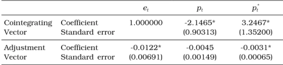
Table 2 shows the estimation results of the PPP forecasting model.

The VECM is estimated at the ECM lag-length of 2. The cointegrating relationship involves the positive coefficient on the foreign price level and the negative coefficient on the domestic price level. The coefficient estimates and the corresponding standard errors support the PPP principle. The cointegrating coefficients look different from the PPP relation;

e_t－p_t＋p_t^*. However, the hypothesis testing for the coefficient restriction (1,－1, 1) cannot be rejected. The long-run relationship is stationary;

hence, the nominal exchange rate is associated positively with the domestic price level and negatively associated with the foreign price level.

The adjustment coefficient of the nominal exchange rate equation is both negatively and statistically significant. The nominal exchange rate responds negatively to the long-run equilibrium error, and the nominal exchange rate is adjusted if the actual level deviates from the long-run equilibrium level. The value of the adjustment coefficient shows that the exchange rate responds slowly to the PPP disequilibrium errors.

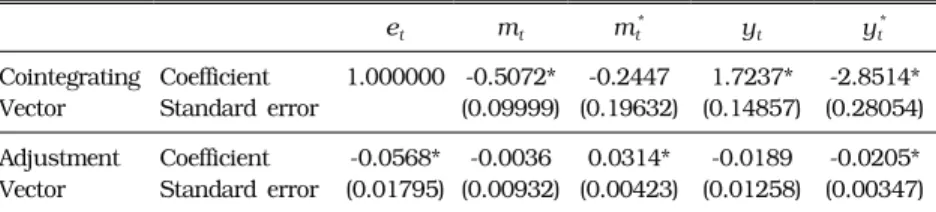
The estimation results of the EQ long-run relationship are shown in Table 3. The cointegrating relationship entails positive coefficients on the nominal exchange rates and domestic income and negative coefficients on the domestic money stock and foreign income. The coefficient

(13)

e_t m_t m_t^* y_t y_t^* Cointegrating

Vector

1.000000 -0.5072*

(0.09999)

-0.2447 (0.19632)

1.7237*

(0.14857)

-2.8514*

(0.28054) Adjustment

Vector

-0.0568*

(0.01795)

-0.0036 (0.00932)

0.0314*

(0.00423)

-0.0189 (0.01258)

-0.0205*

(0.00347) Note: * 5% significant.

TABLE 3

ESTIMATION OF EQ LONG-RUN RELATIONSHIP

on the US money stock is estimated to have a negative value but is not statistically significant.

The nominal exchange rates increase when the domestic money supply increases, thus raising the long-run equilibrium level of exchange rates. Additionally, the increase in domestic income lowers the exchange rates because domestic income is associated negatively with the equilibrium exchange rates. The adjustment coefficient of the exchange rate equation is significantly negative. Thus, the nominal exchange rates adjust to restore the equilibrium when the actual level deviates from the equilibrium level based on the EQ model.

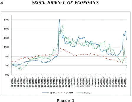
Figure 1 demonstrates the long-run equilibrium exchange rates based on the PPP and EQ relationships. The overvaluation of the Korean won to the US dollar occurs in the 1990s prior to the 1997 Asian crisis. After the crisis, the Korean won is steadily undervalued when the PPP relationship is considered. However, we can observe the overvaluation of the Korean won after the crisis and prior to the global financial crisis of 2008 in terms of the EQ long-run equilibrium. The undervaluation of the Korean won has been noted based on the PPP and EQ long-run relationship since 2008.

The long-run equilibrium exchange rate based on the PPP exhibits a long-range swing as the domestic and foreign prices evolve slowly. The long-run exchange rate based on the EQ model traces the spot exchange rate more closely. The fundamental variables, such as domestic and foreign money supply and income, respond to disequilibrium errors, which strengthen the adjustment process.

The long-run equilibrium relationship of the real exchange rates may be disrupted as a result of policy misalignment. In the 1990s, the government maintained the exchange rate policy to sustain the strength of the domestic currency. However, the increase in the money supply and

(14)

FIGURE 1

LONG-RUN EQUILIBRIUM EXCHANGE RATES

the decline in the economic growth rate amplified the overvaluation of the won. The flip of a swing in the Asian financial market resulted in the Korean financial crisis of 1997.

C. Stability Testing

The persistence of disequilibrium in real exchange rates can be gen- erated as a result of the instability of the long-run relationship. The tests for stability in the cointegrating vector are conducted using the Ave-LM, Exp-LM, and Sup-LM statistics provided by Seo (1998).

As presented in Table 4, the test statistics for structural change in the PPP relationship is smaller than the 5% critical values. Thus, the long-run stability of the PPP equilibrium relationship cannot be rejected.

The stability of the adjustment vector for the PPP relationship is also observed. Figure 2 shows the time plot of the LM statistics. The LM statistics achieves its peak near the 1997 Asian crisis, but the value is smaller than the 5% critical value of the Sup-LM statistic. As reported in Table 4, the tests for stability in the cointegrating relationship of the equilibrium model demonstrate that the Ave-LM, Exp-LM, and Sup-LM statistics do not exceed the 5% critical value.

Figure 3 shows the time plot of the LM statistics for stability in the long-run relationship of the EQ forecasting model. The LM statistics

(15)

Ave-LM Exp-LM Sup-LM Statistic 5% c.v. Statistic 5% c.v. Statistic 5% c.v.

PPP Cointegrating Vector

3.6642 4.32 2.3874 3.24 7.8408 12.55

Adjustment Vector

1.2006 6.07 0.8879 4.22 6.3097 14.15

Joint 4.8648 8.74 3.1344 6.13 14.1504 18.71

EQ Cointegrating Vector

7.4099 7.47 4.0652 5.20 11.7254 17.13

Adjustment Vector

10.0693 9.01 5.9491 6.13 15.4751 18.35

Joint 17.4792 14.27 9.9515 9.48 23.7127 26.11

* Asymptotic critical values are provided by Andrews (1993) and Seo (1998).

TABLE 4 TESTING FOR STABILITY

fluctuate below the 5% critical value of the Sup-LM statistic, demon- strating the long-run stability of the equilibrium relationship. However, the adjustment vector reveals instability if the Ave-LM statistics is employed.

D. Regime-dependent Persistence

The persistence of disequilibrium errors in real exchange rates may be associated with regime-dependent persistence. Table 5 summarizes the testing for the regime-dependent persistence of real exchange rates.

The Sup-LM statistics is computed to test for the null hypothesis of linearity against asymmetric adjustment, as provided by Hansen and Seo (2002). The long-run PPP relationship entails the Sup-LM statistics of 110.871, with a p-value of 0.000. Thus, the mean reversion behavior varies according to the state, determined by the magnitude of the PPP disequilibrium errors. The response of the exchange rates to the EQ long-run relationship also reveals an asymmetric adjustment. The Sup- LM statistics is computed at 142.286, which is larger than the 5% critical value.

The regime-dependent persistence behavior of real exchange rates is estimated in Table 6. The rate of adjustment in the linear model is constant and independent of the history. The rate of adjustment in the threshold model varies with the size and sign of the disequilibrium

(16)

FIGURE 2

STABILITY TESTS OF THE PPP FORECASTING MODEL

(1980:01-2009:06)

Sup-LM 5% c.v. p-value

PPP EQ

110.871 142.286

91.844 135.916

0.000 0.011 TABLE 5

TESTING FOR ASYMMETRIC ADJUSTMENT

(17)

FIGURE 3

STABILITY TESTS OF THE EQ FORECASTING MODEL (1980:01-2009:06)

errors. In the left-tail regime, wt－1≤γ1, the adjustment coefficient is both negative and significant. When the disequilibrium errors are smaller than the threshold value γ1, the nominal exchange rates respond to the disequilibrium errors and revert to the equilibrium. The left-tail regime corresponds to the state when the exchange rate is lower than the long- run equilibrium. Thus, the over-valuation of the Korean won is likely to disappear rapidly when the magnitude exceeds the threshold value.

However, in the mid regime, γ1＜w_t－1≤γ2, the adjustment coefficient

(18)

Adjustment

Coefficient Standard Error Log-Likelihood

PPP

Linear Model -0.0131 0.0072 4942.2204

Threshold Model wt－1≤γ1

-0.0678 0.0278

5078.4339 γ1＜wt－1≤γ2 0.0291 0.0179

γ2＜wt－1 -0.0026 0.0415

γ1＝-0.2758 γ2＝0.0849

P(wt－1≤γ1)^＝ 0.1029

P(γ1＜wt－1≤γ2)^＝ 0.5029

P(γ2＜wt－1)^＝ 0.3943

EQ

Linear Model -0.0397 0.0203 4717.7447

Threshold Model wt－1≤γ1

-0.5044 0.2889

4923.4990 γ1＜wt－1≤γ2 -0.0125 0.0163

γ2＜wt－1 -0.1557 0.0626

γ1＝-0.1424 γ2＝0.1494

P(wt－1≤γ1)^＝ 0.1053

P(γ1＜wt－1≤γ2)^＝ 0.7851

P(γ2＜wt－1)^＝ 0.1096 TABLE 6

ESTIMATION OF ASYMMETRIC ADJUSTMENT

has a positive, albeit insignificantly positive, value. The nominal exchange rates do not respond to the disequilibrium errors, and disequilibrium persists in the mid regime. In the right-tail regime, wt－1 ＞γ2, the adjustment coefficient has a negative value but is not significant. If the exchange rates are undervalued, the rate of adjustment will not be large enough to restore the equilibrium. The right-tail regime corresponds to the state in which the exchange rate is higher than the long-run equilibrium. Thus, the undervaluation of the Korean won—US dollar exchange rate is likely to persist. The mean reversion behavior demonstrates path dependence.

The log-likelihood of the linear model is significantly smaller than that of the threshold cointegration model. Table 5 documents the evidence of the threshold effect. The movement of exchange rates is largely consistent with the regime-dependent mean reversion behavior. The probability of remaining at the mid regime is estimated at 50.3% in the PPP forecasting model and at 78.5% in the EQ forecasting model. The dur- ation of disequilibrium in the mid regime is far longer than that in the

(19)

RMSE MAE Baseline Random Walk 44.8019 1.0000 18.9198 1.0000

PPP ECM

Instability Threshold Effect

36.6404 36.0521 26.0716

0.8178 0.8047 0.5819

17.2240 17.1491 16.0169

0.9104 0.9064 0.8466

EQ ECM

Instability Threshold Effect

38.7870 38.0181 28.3892

0.8657 0.8486 0.6337

18.0752 18.7510 16.8231

0.9554 0.9911 0.8892 PPP & EQ

Combination ECM*

Instability**

Threshold Effect***

36.5880 35.8322 25.1701

0.8167 0.7998 0.5618

17.0312 16.7402 15.4729

0.9002 0.8848 0.8178

* weight^＝0.8679; ** weight^＝0.7616; *** weight^＝0.6813 TABLE 7

FORECASTING ACCURACY (1990:04-2009:06)

tail regimes. Thus, the persistence of disequilibrium prevails in the mid regime, and the transition to the left- and right-tail regimes is likely to occur with a relatively low probability.

E. Prediction Accuracy

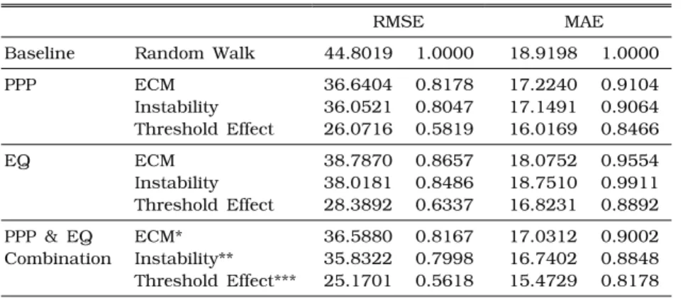
Table 7 summarizes the prediction accuracy measured in terms of the root mean squared errors (RMSE) and mean absolute errors (MAE).

The baseline forecast assumes that future changes in the exchange rates are unpredictable. The ECM forecast is made on the VECM, with the long-run relationship of the PPP and EQ. The forecast instability assumes structural changes in the parameters. The break point of instability is estimated to occur in November 1997, thus corresponding to the 1997 Asian financial crisis, for both the PPP and the EQ forecasting models. The forecast threshold effect is based on the threshold cointegration model.

For the forecasting model with the PPP equilibrium relationship, the ECM forecast improves the prediction accuracy by approximately 18.2%

in terms of the RMSE and by approximately 9% in terms of the MAE relative to the baseline forecast. The forecast instability provides no significant gains in the prediction accuracy in relation to the forecast ECM.

However, the forecast threshold effect demonstrates a huge amount of gain in prediction accuracy. Compared with the ECM forecast, the forecast threshold effect reduces the RMSE by 23.59% and the MAE by 6.38%. When composing the forecast combination using the forecast

(20)

instability and the threshold effect, the optimal weight is computed by the grid search method. The optimal weight is 0 for the forecast instability and 1 for the forecast threshold effect. Thus, the hysteresis of real exchange rates is associated with asymmetric mean reversion, which reflects the regime-dependent nature of the persistence of the PPP disequilibrium errors. The parametric instability does not help in iden- tifying the source of the hysteresis. Table 7 shows the evaluation of the forecast threshold cointegration (TC) against structural change (ST). The prediction accuracy of the forecast TC outperforms the forecast ST. Thus, the hysteresis is related to the nonlinear mean reversion. The evidence of permanent change in the long-run relationship is not supported.

As revealed in Table 7, forecasts with the EQ relationship show similar results. The forecast instability provides no gains in prediction accuracy.

The forecast threshold effect ushers in significant gains in reducing the prediction errors. The forecast combination of two forecasts based on the threshold effect of PPP and that of EQ results in improvements in prediction accuracy.

Table 7 also provides the prediction accuracy of the forecast combination. The forecast combination of two forecasts based on the threshold effect of PPP and that of EQ improves the prediction accuracy. As the PPP forecast is suitable for long-term forecasting, the forecast combination may improve the EQ forecast, which is adequate for short-term exchange rate forecasting. The optimal weight is selected by applying the grid-search method to Equation (13).

V. Concluding Remarks

According to the PPP, real exchange rates are stationary and neces- sitate mean-reversion behavior. Furthermore, the principle of the long- run neutrality of money predicts that real exchange rates evolve independently of unanticipated nominal shocks. However, the information contents of the PPP can be influenced by the hysteresis. In the current study, a statistical assessment of hysteresis in the Korean won—US dollar exchange rates has been conducted, and the forecasting combination as a means to identify hysteresis, has been proposed. For the period during which the hysteresis influenced the exchange rates, the improvement in forecasting accuracy appears to be pronounced.

The predictability of exchange rates has been assessed in a number of previous studies, including that of Meese and Rogoff (1983). The

(21)

unpredictability of the PPP has been previously attributed to sticky prices, as in the overshooting hypothesis of Dornbusch (1976). The current paper relates the unpredictability to the hysteresis in real exchange rates. The hysteresis in the Korean won—US dollar exchange rate may originate from the permanent instability of the long-run relationship or from the regime-dependent persistence. The persistence of disequilibrium in real exchange rates may be the result of the instability of the long- run relationship. The tests for stability in the cointegrating relationship of the EQ model reflect the long-run stability of the equilibrium relationship. However, the evolution of real exchange rates is path dependent based on the threshold cointegration. Thus, the prolonged disequilibrium in the exchange rate can be attributed to the path-dependent persistence. We have incorporated the behavior in empirical analysis and obtained a forecast of exchange rates that outperforms the conventional forecasts.

As the exchange rates reveal more volatility, and disequilibrium errors are increasingly prolonged, our analysis techniques can be applied to the hysteresis of other exchange rates. Although the threshold cointegration model has been proposed to explain the regime-dependent persistence, other nonlinear methods can be utilized to evaluate the hysteresis of real exchange rates. However, these issues will have to be explored in future studies.

(Received 29 June 2010; 17 February 2011; Accepted 7 March 2011) References

Andrews, D. “Tests for Parameter Instability and Structural Change with Unknown Change Point.” Econometrica 61 (No. 4 1993): 821-56.

Baldwin, R. E., and Lyons, R. K. “Exchange Rate Hypothesis? Large versus Small Policy Misalignments.” European Economic Review 38 (No. 1 1994): 1-22.

Bilson, J. “The Monetary Approach to the Exchange Rate: Some Empirical Evidence.” IMF Staff Papers 25 (No. 1 1978): 48-75.

Diebold, F., and Nason, J. “Nonparametric Exchange Rate Prediction?”

Journal of International Economics 28 (Nos. 3-4 1990): 315-32.

Dixit, A. “Hysteresis, Import Penetration, and Exchange Rate Pass- Through.” Quarterly Journal of Economics 104 (No. 2 1989): 205- 28.

(22)

Dornbusch, R. “Expectations and Exchange Rate Dynamics.” Journal of Political Economy 84 (No. 6 1976): 1161-76.

Engle, C. “Can the Markov Switching Model Forecast Exchange Rates?”

Journal of International Economics 36 (Nos.1-2 1994): 151-65.

Engle, C., and Hamilton, J. “Long Swings in the Dollar: Are They in the Data and Do Markets Know It?” American Economic Review 80 (No. 4 1990): 689-713.

Frenkel, J. A. “A Monetary Approach to the Exchange Rate: Doctrinal Aspects and Empirical Evidence.” Scandinavian Journal of Economics 78 (No. 2 1976): 200-24.

Hansen, B. E. “Least-Squares Forecast Averaging.” Journal of Econometrics 146 (No. 2 2008): 81-7.

________. “Averaging Estimators for Regressions with Possible Structural Break.” Econometric Theory 25 (No. 6 2009): 1498-514.

Hansen, B. E., and Seo, B. “Testing for Two-Regime Threshold Cointegration in Vector Error Correction Models.” Journal of Econometrics 110 (No. 2 2002): 293-318.

Lucas, R. “Interest Rates and Currency Prices in a Two-Country World.”

Journal of Monetary Economics 10 (No. 3 1982): 335-59.

Mark, C. N. “Exchange Rates and Fundamentals: Evidence on Long- Horizon Predictability.” American Economic Review 85 (No. 1 1995): 201-18.

Meese, R., and Rogoff, K. “Empirical Exchange Rate Models of the 1970's: Do They Fit Out of Sample?” Journal of International Economics 14 (Nos. 1-2 1983): 3-24.

Meese, R. A., and Rose, A. K. “An Empirical Assessment of Nonlinearities in Models of Exchange Rate Determination.”

Review of Economic Studies 58 (No. 3 1991): 603-19.

Meese, R., and Singleton, K. “On Unit Roots and the Empirical Modeling of Exchange Rates.” Journal of Finance 37 (No. 4 1982): 1029- 35.

Michael, P., Nobay, A. R., and Peel, D. A. “Transactions Costs and Nonlinear Adjustment in Real Exchange Rates: An Empirical Investigation.” Journal of Political Economy 105 (No. 4 1997):

862-79.

Mizrach, B. “Multivariate Nearest-Neighbor Forecasts of EMS Exchange Rates.” Journal of Applied Econometrics 7 (December 1992): 151- 63.

Mussa, M. “The Exchange Rate, the Balance of Payments, and Monetary and Fiscal Policy under a Regime of Controlled Floating.”

(23)

Scandinavian Journal of Economics 78 (No. 2 1976): 229-48.

Obstfeld, M., and Taylor, A. M. “Nonlinear Aspects of Goods-Market Arbitrage and Adjustment: Heckscher’s Commodity Points Revisited.” Journal of the Japanese and International Economies 11 (No. 4 1997): 441-79.

Seo, B. “Tests for Structural Change in Cointegrated Systems.”

Econometric Theory 14 (No. 2 1998): 222-59.

Stockman, A. “A Theory of Exchange Rate Determination.” Journal of Political Economy 88 (No. 4 1980): 673-98.

Taylor, M. P., Peel, D. A., and Sarno, L. “Nonlinear Mean Reversion in Real Exchange Rates: Toward a Solution to the Purchasing Power Parity Puzzles.” International Economic Review 42 (No. 4 2001): 1015-42.

(24)