Dynamic Relationship between Stock Prices and Exchange Rates: Evidence from Chinese Stock Markets

Abstract

This paper empirically examines the short-run and long-run causal relationship between stock market prices and exchange rates in Chinese stock markets using monthly data from January 2002 to December 2012 retrieved from the National Bureau of Statistics of the People’s Republic of China. Unit root, cointegra- tion tests, vector error correction estimates, block exogeneity Wald tests, impulse responses, variance decomposition techni- ques and structural break tests are employed. This study found 1) long-run causality from exchange rates to stock prices in Chinese stock markets and 2) short-run causality from Japanese yen and Korean won exchange rates to stock prices in the Shanghai Stock Exchange strongly prevails while in the Shenzhen Stock Exchange weakly prevails . The impact of the global financial crisis from 2007 to 2009 on Chinese stock mar- kets was insignificant.

Keywords: Stock Prices; Exchange Rates; Cointegration;

Granger Causality; Structural Breaks; China JEL Classification: E44, F31, F37, G01, G15

1. Introduction

The relationship between exchange rates and stock prices has significant implications, especially from the viewpoint of re- cent large cross-border movement of funds and investments.

Two theories about the dynamic relationship between exchange rates and stock prices are the traditional approach and portfolio approach. These approaches have long been discussed but have not yet resulted in consensus. The traditional approach

* Administrative Sciences Department, Metropolitan College, Boston University [808 Commonwealth Avenue, Boston, MA 02215, USA Tel:

(+1 617) 358-5627 Fax: (+1 617) 353-6840 E-mail: [email protected]]

** Administrative Sciences Department, Metropolitan College, Boston University [808 Commonwealth Avenue, Boston, MA 02215, USA Tel:

(+1 617) 353-3016 Fax: (+1 617) 353-6840 Email: [email protected] and [email protected]]

claims that depreciation of the domestic currency makes local firms more competitive, leading to an increase in their exports and consequently higher stock prices. This implies a positive correlation between exchange rates and stock prices. The tradi- tional approach suggests that the fluctuation of exchange rates lead to the changes in stock prices. On the contrary, the portfo- lio approach argues that an increase in stock prices induces in- vestors to demand more domestic assets and thereby causes an appreciation in the domestic currency. Thus, changes in stock prices lead to fluctuation of exchange rates and that they are negatively related.

Stock prices, generally interpreted as the present values of future cash flows of firms, react to exchange rate changes and form the link among future income, interest rate innovations, current investment and consumption decisions (Zhao, 2010). In the floating exchange rate system, the exchange rate is essen- tially determined by a country's current account balance or trade balance. As a result, the exchange rate fluctuation affects inter- national competitiveness and trade balance to some extent.

Consequently, it affects real income and stock prices, especially the stock price of export oriented enterprises. Flow-oriented model (Dornbusch & Fisher, 1980) claims a positive linkage be- tween exchange rates and stock prices. Local currency depreci- ation would lead to a greater competitiveness of domestic firms given that their exports will be cheaper in international trade.

Higher exports will increase the domestic income and hence the firms’ stock prices will go up since they are evaluated as the present value of the firms’ future cash flows.

The stock-oriented model (Branson, Halttunen, & Masson, 1977) of exchange rates specifies the exchange rate as serving to equate the supply and demand for assets such as stocks and bonds. This model determines the exchange rate dynamics by giving the capital account a pivotal role. Since the values of financial assets are determined by the present values of their future cash flows, expectations of relative currency values play a considerable role in price movements of the financial assets.

Therefore, stock price innovations may affect, or be affected by, exchange rate dynamics (Zhao, 2010). As a result, if the com- mon factors influence the two variables, stock price innovations may be reciprocally associated with the exchange rate dynamics or be influenced by the exchange rate behavior.

The research goals of this study are to fill the gap in the lit- Print ISSN: 2288-4637 / Online ISSN 2288-4645

doi: 10.13106/jafeb.2014.vol1.no1.5.

Dynamic Relationship between Stock Prices and Exchange Rates: Evidence from Chinese Stock Markets

1)

Jung Wan Lee*, Tianyuan Frederic Zhao**

[Received: November 1, 2013 Revised: February 2, 2014 Accepted: February 15, 2014]

erature and to provide additional evidence on both the short-run and long-run causal relationship between exchange rates and stock prices in Chinese stock markets. The study begins by in- vestigating how information is transmitted between these eco- nomic variables through long-run and short-run price interactions.

2. Conceptual Background and Hypotheses

Previous studies have addressed different findings regarding the causal relations between stock prices and exchange rates in various countries. For example, Nieh and Lee (2001) found no long-run relationship between stock prices and exchange rates in the Group-7 countries. Yau and Nieh (2006) suggested no clear long-run relation between the new Taiwan dollar and the Japanese yen exchange rates and the stock prices of Taiwan and Japan. Zhao (2010) did not find stable long-run relationship between Chinese yuan real effective exchange rates and stock prices. Ramasamy and Yeung (2002) indicated inconsistent re- sults for bidirectional causality between stock prices and ex- change rates for six Asian countries over the period of 1995 and 2001. Kutty (2010) found that stock prices Granger caused exchange rates in the short run but there was no long-run sig- nificant relationship in Mexico between January 1989 and December 2006. Other studies from Griffin and Stulz (2001), Fernandez (2006), Fernandes (2009), Hartmann and Pierdzioch (2007), and Zhao (2010) suggest no relationship between ex- change rates and stock prices. On the other hand, the long-run relationship has been confirmed in some studies. Nieh (2009) found a long-run and asymmetric causal relationship between the exchange rates of new Taiwan dollar and Japanese yen and their stock prices in Japan and Taiwan. Whether empirically or theoretically, the above studies have suggested a significant relationship between exchange rates and stock prices, but the results have been mixed for the sign and causal direction be- tween exchange rates and stock prices. Thus, the following hy- pothesis is advanced:

Hypothesis 1: Exchange rates lead stock price dynamics in the long-run in Chinese stock markets.

In addition, Phylaktis and Ravazzolo (2005) employed co- integration and multivariate Granger causality tests that resulted in positive long-run and short-run causality between stock prices and exchange rates in some Pacific Basin countries. Aloui (2007) indicated that movements of stock prices affect the ex- change rate dynamics for the two periods pre- and post-Euro in the United States and Western European markets. Pan, Fok and Liu (2007) reported a causal relation from exchange rates to stock prices for East Asian countries. Yang and Doong (2004) suggested exchange rate changes directly impacted fu- ture changes of stock prices for the Group-7 countries from 1979 to 1999. Nandha and Hammoudeh (2007) argued that stock prices were affected by changes in the exchange rate for

nine Asia-Pacific countries while Wu (2001) showed Singapore dollar exchange rates Granger caused stock prices. Further re- search emphasizing positive relationship between exchange rates and stock prices can be found in Chiang and Yang (2003), Ratanapakorn and Sharma (2007), Kolari, Moorman, and Sorescu (2008), Aydemir and Demirhan (2009), Ning (2010), Chu and You (2011), and Eichler (2011). Mun (2007) specified that higher exchange rate variability mostly increases local stock market volatility, but decreases volatility for the United States stock markets. Exchange rate exposure has negative and sig- nificant impact on emerging market stock returns in a study by Chue and Cook (2008) while the S&P 500 stock price is neg- atively related to the real exchange rates in Kim (2003)’s research. Thus far, the relationship between stock prices and exchange rates is still inconclusive. Therefore, further study is needed to elucidate the causality between stock prices and ex- change rates. Hence:

Hypothesis 2: The nominal exchange rates of Chinese yuan per U.S. dollar, Euro, Japanese yen and South Korean won, respectively, affect stock price dy- namics in the short-run.

The linkage between exchange rates and stock prices vary across economies with respect to exchange rate regimes, the trade size, the degree of capital control and the size of equity market (Pan, Fok & Liu, 2007). Mercereau (2006) suggested that the financial structure of an equity market influenced its real exchange rate, as well as the volatility of this exchange rate, whereas Walid, Chaker, Masood and Fry (2011) asserted that the stock price volatility responded asymmetrically to events in the foreign exchange market. Diamandis and Drakos (2011) found that there is a significant long-run relationship between the local stock market and the exchange rate market, but that the stability of the relationship is affected by financial and cur- rency shocks such as the Mexican currency crisis of 1994 and the global financial crisis of 2007 to 2009. In addition, during the creation of the Mercosur between Argentina, Brazil, Paraguay and Uruguay in Latin American countries, this process led to the local currency devaluation. These exchange rate movements have substantial negative impact on the respective stock prices (Allegret & Sand-Zantman, 2009; Alvarez-Plata &

Schrooten, 2004; Camarero, Flores Jr. & Tamarit, 2006).

Hatemi-J and Roca (2005) reported that the two variables are significantly linked in the non-crisis period, but not at all during the crisis period for ASEAN countries. Exchange rates and stock prices are correlated in a complicated manner (Kim, Yoon

& Kim, 2004: Tastan, 2006). As such, market interactions may destabilize stock markets, but may also play a stabilizing effect on the exchange rate market (Dieci & Westerhoff, 2010). Thus, the following hypothesis is developed:

Hypothesis 3: The global financial crisis of 2007-2009 has im-

pacted the stock price dynamics in Chinese

stock markets.

3. Empirical Specification

Engle and Granger (1987) and Granger (1988) specify that if two or more variables are cointegrated, there always exists a corresponding error correction term in which the short-run dy- namic of the variables in the system are influenced by the devi- ation from equilibrium. In this case, a vector error correction (VEC) model is formulated to reintroduce the information lost in the differencing process, thereby capturing long-run dynamics as well as short-run dynamics. The VEC model implies that changes in one variable are a function of the level of dis- equilibrium in the cointegrating relationship (captured by the er- ror correction term), as well as changes in other explanatory variables. Thus, the VEC model is useful for capturing both the long-run and the short-run dynamics when the variables are cointegrated.

Equations 1 and 2 illustrate multivariate vector autoregressive models with the error correction term. In this study, equations 1 and 2 will be used to test long-run and short-run Granger cau- sation from exchange rates to stock prices in Chinese stock markets.

where:

indicates the difference operator;

Δ

ln indicates the logarithm;

is the deterministic component;

α

, , and denote the parameters to be estimated;

β θ ζ

et follows stationary random errors with mean zero, that is, white noise;

j is the lag length;

t represents 1, 2, 3, , n observation; …

ECTtis the error correction term obtained from the cointegrat- ing vectors deriving from the long-run cointegrating relationship via the Johansen maximum likelihood procedure.

SSE denotes the index of overall market value of listed stocks in the Shanghai Stock Exchange.

SZSE denotes the index of overall market value of listed stocks in the Shenzhen Stock Exchange.

INF refers to the inflation rate.

INT represents the interest rate.

M2 is the broad definition of money supply.

POL refers to the policy shock dummy. It is used as a proxy for monetary policy changes, for example, implementing the managed floating exchange rate system in July 2005 in China.

The long-run causality is indicated by the significance of t-sta- tistics of the lagged error correction term (i.e. by testing null hy- pothesis: ζ = 0). The asymptotic variance of the estimator is es - timated so that the t-statistics have asymptotic standard normal distribution. Asymptotic t-statistics can be interpreted the same way as t-statistics. They are used to interpret the statistical sig- nificance of coefficients of the lagged error correction term.

4. Data and Methodology

This section describes the data and outlines the methodology used in the selection of indicators and the normalization of data.

The sample is restricted to the period in which monthly data are available from January 2002 to December 2012 (132 ob- servations). All of monthly time series data below are collected and retrieved from the National Bureau of Statistics of the People’s Republic of China (2013), the Shanghai Stock Exchange (2013), and the Shenzhen Stock Exchange (2013).

4.1. Endogenous Variables

Shanghai Stock Exchange. The Shanghai Stock Exchange Composite Index (symbol: SSE) is used as a proxy of Chinese stock market prices. The index is the most commonly used in- dicator to reflect the Shanghai Stock Exchange’s market per- formance and is a capitalization weighted index. The index tracks the daily price performance of all A-shares and B-shares listed on the Shanghai Stock Exchange (2013). The index was developed on December 19, 1990 as the base day and the to- tal market capitalization of all the listed stocks on the same base period, with a base of 100 points. It was published from July 15, 1991 and since then it becomes the most widely used index in China’s securities markets. The index data is collected and retrieved from the Shanghai Stock Exchange Monthly Statistics publication, sponsored by the Shanghai Stock Exchange (2013). Monthly average of this index is used in this study.

Shenzhen Stock Exchange. The Shenzhen Composite Index (symbol: SZSE) is used as another proxy of Chinese stock mar- ket prices. This index is the most commonly used indicator to reflect the Shenzhen Stock Exchange’s market performance and is an actual market capitalization weighted index, with no free float factor, that tracks the stock performance of all the A-share and B-share lists on the Shenzhen Stock Exchange (2013). The index was developed on April 3, 1991 with a base price of 100.

The index was scaled down by a factor of 1000 as the base

day of July 20, 1994 and was introduced on January 23, 1995.

The index data is collected and retrieved from the Shenzhen Stock Exchange Monthly Statistics publication, sponsored by the Shenzhen Stock Exchange (2013). Monthly average of this in- dex is used in this study.

Foreign Exchange Rates. Based on the volume of interna- tional trade with China, four major exchange rates are selected:

Chinese yuan per U.S. dollar (USD), Euro (EUR), Japanese yen (JPY) and South Korean won (KRW), respectively. The time ser- ies data is a monthly adjusted average. In effect, USD, EUR, JPY and KRW are the logarithm of the nominal exchange rate of Chinese yuan per U.S. dollar, Euro, Japanese yen and South Korean won, respectively.

Macroeconomic Variables. Money supply (M2), inflation rate, and short-run interest rate are included in the model to address the omitted variable bias. In the empirical model, M2 is the log- arithm of changes in the broad definition of money supply.

Inflation is the logarithm of the first difference of the consumer price index, an inflation rate. Interest is the logarithm of the short-term (1 year) interest rate.

Monetary Policy Shock. A monetary policy shock refers to the sudden release of price and currency controls, withdrawal of state subsidies, and immediate trade liberalization within a coun- try, usually also including large scale privatization of previously public owned assets. In July 2005, the Chinese central bank, People’s Bank of China, initiated an exchange rate system re- form, which terminated the fixed floating exchange rate system and implemented the managed floating exchange rate system.

Since that time, the Chinese yuan exchange rate has become more flexible to some extent and keeps a major trend of appre- ciation against U.S. dollar. It is noteworthy that Chinese stock markets performed remarkably well in the year of 2005 and started to experience greater volatility than ever before in the managed floating exchange rate system. It brings some doubt whether there is an interrelationship between stock prices and exchange rates in China. A dummy variable with a value of 0 will cause the variable’s coefficient to disappear, and a dummy with a value 1 will cause the coefficient to act as a supple- mental intercept in the regression model. Hence, the policy shock variable equals 1 if the period falls on after July 2005 and 0 otherwise.

4.2. Exogenous Variable

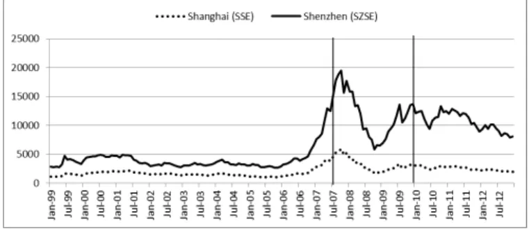
The Global Financial Crisis (2007-2009) Shock. The global fi- nancial crisis of 2007-2009 may cause a structural break in the trend of stock prices in Chinese stock markets, see Figure 1.

Because the global financial crisis would introduce some changes in the implementation of monetary policy, for example, from money targeting to interest rate targeting, this would in- troduce substantial instability in the system. A dummy is used to examine the impact of the global financial crisis of 2007-2009 on Chinese stock market. However, the dummy here is used as an exogenous variable because it is assumed not to be system- atically affected by changes in the endogenous variables of the

model. A dummy variable with a value of 0 will cause the varia- ble’s coefficient to disappear, and a dummy with a value 1 will cause the coefficient to act as a supplemental intercept in the regression model. Hence, the global financial crisis shock varia- ble equals 1 if the period falls on from August 2007 to December 2009 and 0 otherwise.

<Figure 1> Trends of Chinese Stock Market Prices (2007/08 – 2009/12)

Normalization and Transformation. The normalization of the data is necessary to transform the values to the same unit of measurement since stock market indexes are presented as the base value of 100, 1000, or 2000 respectively, while exchange rates are presented in Chinese yuan. Therefore, transformation into a natural log mitigates possible distortions of dynamic prop- erties of the series. Log transformation is a preferred method since each resulting coefficient in regression equation represents elasticity that is the ratio of the incremental change of the loga- rithm of a function with respect to an incremental change of the logarithm of the argument.

Selected tests on time series data as prescribed in the refer- ences in each section below are necessary for statistical accu- racy and to avoid spurious results. To ascertain the order of in- tegration of the variables, this study applied the augmented Dickey-Fuller (Dickey & Fuller, 1981) unit root test and the Phillips Perron (Phillips & Perron, 1988) test. The augmented – Dickey-Fuller test assumes the errors to be independent and have constant variance while the Phillips Perron test allows for – fairly mild assumptions about the distribution of errors. The two unit root tests are carried to test the null hypothesis of the unit root in the level and the first difference of the variables. All test equations were tested by the method of least squares, including an intercept but no time trend in the model. In the unit root tests, an optimal lag in the tests is automatically selected based on Schwarz information criterion and the lag length in the tests is automatically selected based on the Newey-West estimator using the Bartlett Kernel function.

Table 1 reports the results of the two unit root tests. Table 1

indicates the null hypothesis of a unit root cannot be rejected in

the level of SSE, SZSE, USD, EUR, JPY, and KRW, but after

first differencing, all null hypothesis of a unit root is rejected at

the 1% significance level for these variables. The results in

Table 1 unanimously confirm that all variables are integrated of

order one I(1).

<Table 1> Results of Unit Root Test Test

Method Augmented Dickey-Fuller

Test Phillips Perron Test – Variable Level 1

difference Level 1

difference

SSE -1.669 -7.144*** -2.169 -12.203***

SZSE -2.055 -7.076*** -2.075 -11.971***

USD 0.808 -3.827*** 1.383 -11.163***

EUR -1.524 -12.633*** -1.524 -12.635***

JPY -1.257 -10.748*** -1.573 -10.553***

KRW -1.563 -5.897*** -1.453 -8.178***

Inflation -4.016*** -5.082*** -10.193*** -67.917***

Interest -2.037 -8.189*** -1.895 -8.384***

M2 -0.019 -5.049*** -0.001 -12.566***

Probability values for rejection of the null hypothesis of a unit root are employed at the 0.05 level (**, p < 0.05 and ***, p < 0.01).

Cheung and Ng (1998) reported that the Johansen approach is more efficient than the Engle-Granger single equation test method because the maximum likelihood procedure has large and finite sample properties. The Johansen(1988)’s approach derives maximum likelihood estimators of the cointegrating vec- tors for an autoregressive process with independent errors. The Johansen cointegration test represents each variable as a func- tion of all the lagged endogenous variables in the system. It uses two ratio tests, a trace test and a maximum eigenvalue test, to examine the number of cointegration relationships. Both tests could be used to determine the number of cointegrating vectors present, although they do not always indicate the same number of cointegrating vectors. If trace statistics and maximum eigenvalue statistics yield different results, the result of the max- imum eigenvalue test is preferred because of the benefit of car- rying out separate tests on each eigenvalue.

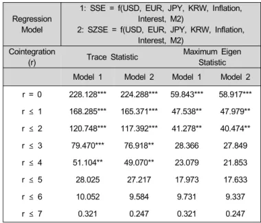
Table 2 reports the results of the Johansen cointegration test.

The test equation is tested by the method of least squares. The regression model allows for a linear deterministic trend in data and includes the intercept but no trend in the vector autore- gressive model. Trace test indicates that at least five cointegrat- ing equations exist at the 0.05 level while maximum eigenvalue test indicates that at least three cointegrating equations at the 0.05 level. Thus, they are statistically significant. Therefore, there exists cointegration between stock prices and foreign ex- change rates in Chinese stock markets. In this case, an unre- stricted vector autoregressive model would not be an effective option for testing the long-run and short-run causality.

<Table 2> Results of Johansen Cointegration Test Regression

Model

1: SSE = f(USD, EUR, JPY, KRW, Inflation, Interest, M2)

2: SZSE = f(USD, EUR, JPY, KRW, Inflation, Interest, M2)

Cointegration

(r) Trace Statistic Maximum Eigen

Statistic Model 1 Model 2 Model 1 Model 2 r = 0 228.128*** 224.288*** 59.843*** 58.917***

r ≤ 1 168.285*** 165.371*** 47.538** 47.979**

r ≤ 2 120.748*** 117.392*** 41.278** 40.474**

r ≤ 3 79.470*** 76.918** 28.366 27.849

r ≤ 4 51.104** 49.070** 23.079 21.853

r ≤ 5 28.025 27.217 17.973 17.633

r ≤ 6 10.052 9.584 9.731 9.337

r ≤ 7 0.321 0.247 0.321 0.247

Probability values for rejection of the null hypothesis of no cointegration are employed at the 0.05 level (**, p < 0.05 and ***, p

< 0.01).

5. Empirical Results and Discussion

Statistical inference is sensitive to parameter instability, serial correlation in residuals and residual skewness. As such Table 3 reports the results of VEC estimates, model diagnostic tests and residual diagnostic tests. There are considerably fewer outliers and the fluctuation bands are smaller (Figure 2). Skewness of the series is not significantly different from a normal distribution.

Histogram normality Jarque-Bera test (null hypothesis: residuals are multivariate normal) is not rejected. Breusch-Godfrey serial correlation Lagrange multiplier or LM test (null hypothesis: no serial correlation at lag order 2 is not rejected.

Heteroskedasticity test (null hypothesis: no autoregressive condi- tional heteroskedasticity or ARCH effect at lag order 1 is not rejected. Thus, this model yields acceptable results.

-3 -2 -1 0 1 2 3

02 03 04 05 06 07 08 09 10 11 12

<Figure 2> Graph of Standardized Residuals

The long-run dynamics is determined by the error correction

term. If the coefficient of the error correction term is significant,

then it indicates the evidence of the long-run causality from the

explanatory variables to the dependent variable. This contains the long-run dynamic information because it is derived from the cointegrating relationship. Recall hypothesis 1 that exchange rates lead stock price dynamics in the long-run. For the long-run dynamics, the result of VEC estimates and Wald tests support hypothesis 1. The null of hypothesis 1 is rejected at the 0.05 level for both the Shanghai Stock Exchange and the Shenzhen Stock Exchange markets. Hence, we found good evi- dence of the long-run causation from exchange rates to stock prices in the Chinese stock markets.

The short-run Granger causality in the VEC model can be tested by the block exogeneity Wald test. The block exogeneity Wald test in the VEC system provides Chi-square statistics of coefficients on the lagged endogenous variables. These are used to interpret the statistical significance of coefficients of the endogenous variables. The hypothesis in this test is that the lagged endogenous variable does not Granger cause the de- pendent variable. Hypothesis 2 states that the nominal exchange rates of Chinese yuan per U.S. dollar, Euro, Japanese yen and South Korea won, respectively, lead stock price dynamics in the short-run. For the short-run dynamics, the results support hy- pothesis 2 for Japanese yen and Korean won. The null of hy- pothesis can be rejected at the 0.05 level, which means the

nominal exchange rates of Chinese yuan per Japanese yen and Korean won strongly lead stock price dynamics in the short run – in the Shanghai Stock Exchange market while weakly lead stock price dynamics in the Shanghai Stock Exchange market.

The investigation of hypothesis 3 that the global financial cri- sis of 2007-2009 has impacted the stock price dynamics in the Chinese stock markets results in no rejection of its null hypothesis. In other words, it is statistically insignificant. There is no evidence of the structural break from the global financial crisis shock to stock price dynamics in the Chinese stock markets. An external shock neither affects changes in the en- dogenous variables nor cause instability in the cointegrating vec- tor in the VEC system. Thus, the endogenous variables are de- termined by their own dynamics in the model. The VEC model excluding the structural shock exogenous (dummy) variable is stable and valid for testing the model.

In addition to the findings corresponding to the above hypoth- eses, the impulse responses and variance decomposition may be noteworthy in their impact. A shock to the j-th variable not only directly affects the j-th variable but is also transmitted to all of the other endogenous variables through the dynamic (lag) structure of the vector autoregressive. The effects of the shocks on the endogenous variables can be assessed by estimating im-

<Table 3> Results of Vector Error Correction(VEC) Estimates and Wald Tests

VEC Equation 1 VEC Equation 2

Endogenous variables:

Optimal lag order in ( ) Coefficient t-statistics in [ ]

Wald Tests Chi-square statistics

Coefficient t-statistics in [ ]

Wald Tests Chi-square statistics Long-run

dynamics -0.036[-2.811]*** 12.431*** -0.031[-2.823]*** 10.428**

Short-run dynamics

SSE(t-2)

SZSE(t-2) 0.253[2.698]*** 14.888***

0.266[2.897]*** 10.086**

USD(t-1) 1.207[0.719] 3.629 1.573[0.857] 4.075

EUR(t-1) -0.317[-1.202] 1.815 -0.374[-1.292] 0.975

JPY(t-1) -0.752[-2.206]** 9.688** -0.650[-1.726]* 5.192

KRW(t-4) -0.893[-3.016]*** 9.642** -1.051[-3.179]*** 8.059*

Inflation(t-1) -1.721[-1.604] 8.832* -1.913[-1.646] 7.012

Interest(t-1) 0.298[0.826] 2.269 0.228[0.571] 2.013

M2(t-1) 1.290[1.774]* 2.898 1.168[1.447] 1.842

Policy (t-1) 0.083[1.036] 3.903 0.032[0.354] 1.959

Exogenous variables

: determinant

α -0.016[-1.220] -0.009[-0.624]

Dummy 0.054[1.618]

Model diagnostic tests

Dependent variable SSE(t) SZSE(t)

R-squared = 0.220 = 0.210

Adjusted R-squared = 0.154 = 0.143

F-statistic = 3.335*** = 3.145***

Residual diagnostic tests

Histogram normality test Jarque-Bera test statistic

= 4.017 Jarque-Bera test statistic

= 0.159 Breusch-Godfrey serial

correlation LM test F-statistic

(2, 116) = 0.516 F-statistic

(2, 116) = 0.339 Heteroskedasticity test:

ARCH effect F-statistic

(1, 126) = 0.201 F-statistic

(1, 126) = 0.513

The probability value for rejection of the null hypothesis is employed at the 0.05 level (*, p < 0.1; ** p < 0.05; and ***, p < 0.01).

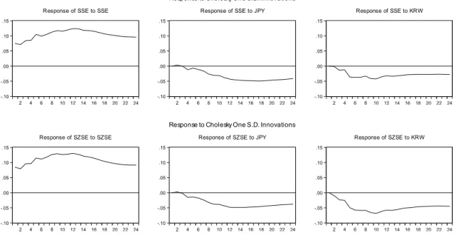
pulse responses and variance decomposition functions. An im- pulse response function traces the effect of a one-time shock to one of the innovations on current and future values of the en- dogenous variables. Since innovations are usually correlated, it may be viewed as having a common component that cannot be associated with a specific variable. In order to interpret the im- pulses, it is common to apply a transformation to the in- novations so that they become uncorrelated. The Cholesky transforming method uses the inverse of the Cholesky factor of the residual covariance matrix to orthogonalize the impulses.

This method imposes an ordering of the variables in the vector autoregressive and attributes all of the effect of any common component to the variable that comes first in the vector autore- gressive system. For stationary vector autoregressive models, the impulse responses should die out to zero and the accumu- lated responses should be asymptote to some constant.

Figure 3 presents the results of the impulse responses of stock prices to Cholesky one standard deviation innovations of three significant endogenous variables: stock price, exchange rate against Japanese yen, and exchange rate against Korean won. The response of stock prices itself to each shock show a positive impact in the first few months, then decline and level off after 12 months. Hence, the impulse response of stock pri- ces is largely determined by its own shock. However, the re- sponses of stock prices to Japanese yen and Korean won show a negative impact in the short-run while widening but leveling off after 12 months. One might expect that the nominal ex- change rate of Chinese yuan to Japanese yen and Korean won has an adverse impact on the Chinese stock market prices as the inflow in portfolio investment from Japan and South Korea plunges when Chinese yuan appreciates against the Japanese yen and the Korean won.

While impulse response functions trace the effects of a shock to one endogenous variable onto the other variable in the vec- tor autoregressive, variance decomposition separates the varia- tion in an endogenous variable into the component shocks to the vector autoregressive. This breaks down the variance of the forecast error for each variable into the components that can be contributed to each of the endogenous variables. Thus, the var- iance decomposition provides information about the relative im- portance of each random innovation in affecting the variables in the vector autoregressive.

Table 4 presents the results of variance decomposition. The reported numbers indicate the percentage of the forecast error in each variable that can be attributed to innovations in other endogenous variables at 24 different horizons from 1 to 24 months ahead or from short-run to long-run. Under SSE and SZSE columns, 100 percent of the variability in SSE and SZSE changes is explained by their own innovations in the first month. Approximately 66 and 62 percent of the variability in SSE (62 and 60 percent in SZSE) is explained by its own in- novations at 12 and 24 months, respectively. With respect to the response of Chinese stock prices to Japanese yen and Korean won exchange rates, zero percent of the variability in SSE and SZSE changes is explained by Japanese yen and Korean won exchange rates in the first month. At 12 and 24 months, approximately 3 and 7 percent of the variability in SSE and approximately 4 and 7 percent of the variability in SZSE, respectively, is explained by Japanese yen exchange rate while they are approximately 5 percent in SSE and 12 percent in SZSE explained by Korean won exchange rate.

-.10 -.05 .00 .05 .10 .15

2 4 6 8 10 12 14 16 18 20 22 24 Response of SSE to SSE

-.10 -.05 .00 .05 .10 .15

2 4 6 8 10 12 14 16 18 20 22 24 Response of SSE to JPY

-.10 -.05 .00 .05 .10 .15

2 4 6 8 10 12 14 16 18 20 22 24 Response of SSE to KRW Response to Cholesky One S.D. Innovations

-.10 -.05 .00 .05 .10 .15

2 4 6 8 10 12 14 16 18 20 22 24 Response of SZSE to SZSE

-.10 -.05 .00 .05 .10 .15

2 4 6 8 10 12 14 16 18 20 22 24 Response of SZSE to JPY

-.10 -.05 .00 .05 .10 .15

2 4 6 8 10 12 14 16 18 20 22 24 Response of SZSE to KRW Response to Cholesky One S.D. Innovations

<Figure 3> Impulse Response of SSE/SZSE to Innovations of JPY and KRW

<Table 4> Variance Decompositions of SSE, SZSE, Japanese Yen, and Korean Won

Period SSE Japanese yen Korean

won SZSE Japanese

yen Korean won

1 100.00 0.00 0.00 100.00 0.00 0.00

2 94.17 0.08 0.01 94.27 0.05 0.66

3 88.78 0.05 0.95 88.34 0.05 2.57

4 83.99 0.50 1.12 83.74 0.65 3.44

5 80.04 0.43 3.63 78.51 0.78 6.66

6 76.70 0.53 5.01 73.80 0.99 9.15

7 73.73 0.76 5.65 70.51 1.33 10.47

8 71.49 1.32 5.61 68.06 1.89 10.93

9 69.37 1.83 5.97 65.80 2.46 11.60

10 67.55 2.23 6.28 63.84 2.87 12.29

11 66.46 2.79 6.15 62.74 3.37 12.41

12 65.80 3.39 5.87 62.16 3.92 12.29

13 65.09 3.93 5.70 61.59 4.38 12.26

14 64.41 4.45 5.56 61.11 4.79 12.23

15 63.95 4.93 5.42 60.85 5.16 12.15

16 63.63 5.37 5.28 60.68 5.48 12.09

17 63.29 5.79 5.17 60.51 5.77 12.05

18 62.97 6.18 5.10 60.34 6.04 12.03

19 62.74 6.52 5.05 60.22 6.26 12.03

20 62.57 6.81 5.01 60.13 6.44 12.06

21 62.43 7.06 5.00 60.05 6.61 12.09

22 62.31 7.27 4.98 59.98 6.75 12.12

23 62.23 7.45 4.98 59.94 6.87 12.17

24 62.17 7.59 4.99 59.90 6.97 12.23

6. Recommendations and Conclusion

This research contributes to the existing literature in three main aspects. First, this research uncovers the fact that there exists long-run causality from exchange rates to stock prices in Chinese stock markets. Second, the paper empirically explores the short-term dynamic relationships between exchange rates and stock prices. The short-run causality from Japanese yen and Korean won exchange rates to Chinese stock prices exists.

Finally, the global financial crisis of 2007-2009 has no impact on the stock price dynamics in the Chinese stock markets. In light of these findings, financial managers can enhance their un- derstanding of the long-term and the short-term movements of exchange rates and stock price dynamics. A better under- standing of these long-term and short-term movements enables financial managers to make well informed investment and finan- cial decisions.

Recommendations can be drawn from the findings presented here. For a long-term perspective, policymakers may consider

the exchange rates as a policy tool aiming at the Chinese stock markets since the results of Granger causality tests show good evidence of the long-run causation from exchange rates such as Chinese yuan per U.S. dollar, Euro, Japanese yen and Korean won to stock prices in the Chinese stock markets. The error correction term of cointegrating equations is statistically sig- nificant, which is negatively associated with stock price dynam- ics in the long-run. One might expect that the appreciation of the nominal exchange rate of Chinese yuan against foreign cur- rencies has an adverse impact on the Chinese stock market pri- ces as the inflow in portfolio investment from foreign investors plunges.

In addition, from a short-term perspective, policymakers may also consider the exchange rates as a policy tool to manage and control the Chinese stock markets since the exchange rate of Chinese yuan per Japanese yen and Korean won, to some extent, would cause an adverse effect on stock prices in China.

This policy would be effective in the short-term and should be evaluated soundly. On the contrary, the results acknowledge that currency volatility of the U.S. dollar and Euro has no Granger causality on stock prices in China. It would appear that this independent behavior of the stock market could be a state of the market liberalization and globalization process for its economy to heal and propel itself toward long-run stability and a better future of the Chinese stock markets.

It is noteworthy that the openness level of Chinese yuan ex- change rates is still low and the Chinese yuan exchange market is under significant influence of the government controlled economy. For example, Chinese yuan can only be exchanged under strict supervision by the state regulator and all the ex- change transactions need to pass the examination and approval before executing. Such regulatory process largely reduces the liquidity and volatility of Chinese yuan exchange markets.

Although the Chinese government has been gradually relaxing the restrictions since the Chinese yuan exchange rate reform (Hu, 2007), there is no tendency that the Chinese yuan ex- change market’s mobility will be improved in the near future.

The Chinese government tends to remain the strict regulations and suppress the Chinese yuan exchange market to some ex- tent through its managed floating exchange rate system. It brings some doubt whether the linkage between stock prices and exchange rates in China can be partially weakened by the government regulations.

It is also noteworthy that Chinese capital markets have been under significant influence of the government controlled economy. The government interferes stock markets not only us- ing diverse monetary policies, but also issuing different industry standards (e.g., China Securities Regulatory Commission, 2013).

For example, the Chinese government highly controls the inflow

of foreign capital investments (Davies, 2013). The barriers that

restrict the capital inflow from foreign capital markets directly in-

to the Chinese capital markets are set up to maintain the

Chinese yuan exchange rate between upper and lower bounds

set by the central bank. This policy deters foreign capital invest-

ments into the Chinese capital markets, especially A-share mar- kets of the Chinese stock markets. Since foreign investors are not allowed to directly invest in the Chinese stock markets, in- direct investments by purchasing financial instruments such as index funds or qualified foreign institutional investor funds are al- ternative options.

That being said, when Chinese yuan exchange markets and Chinese capital markets become more mature and much relaxed government intervention occurs it is possible that the similar re- lationship found from the previous studies (e.g., Kim, 2003; Wu, 2001; Yau & Nieh, 2009) exists in China. Therefore, policy- makers and investors should devote more time and effort ac- quiring not only the information on changes in monetary policy and temporary external shocks in the short-run but also the knowledge and information about the market itself.

Further research may be directed at some of the above issues. The empirical model may be estimated with alternative economic and financial factors or markets. Studies encompass- ing different economies should be conducted where data are available. Such research should contribute toward improving our understanding of the market mechanism and responses of each market to the frequently occurring phenomena of economic and financial crisis, whether regional or global.

References

Allegret, J. P., & Sand-Zantman, A. (2009). Does a monetary union protect against external shocks? An assessment of Latin American integration. Journal of Policy Modeling, 31, 102-118.

Aloui, C. (2007). Price and volatility spillovers between exchange rates and stock indexes for the pre- and post-euro period. Quantitative Finance, 7, 1-17.

Alvarez-Plata, P., & Schrooten, M. (2004). Misleading indicators?

The Argentinean currency crisis. Journal of Policy Modeling, 26, 587-603.

Aydemir, O., & Demirhan, E. (2009). The relationship between stock prices and exchange rates: Evidence from Turkey.

International Research Journal of Finance and Economics, 23, 207-215.

Branson, W., Halttunen, H., & Masson, P. (1977). Exchange rate in the short run: the dollar Deutsche mark rate.

European Economic Review, 10, 303 324. –

Camarero, M., Flores Jr, R. G., & Tamarit, C. R. (2006).

Monetary union and productivity differences in Mercosur countries. Journal of Policy Modeling, 28, 53-66.

Cheung, Y. W., & Ng, L. K. (1998). International evidence on the stock market and aggregate economic activity.

Journal of Empirical Finance, 5, 281-296.

Chiang, T. C., & Yang, S-Y. (2003). Foreign exchange risk pre- miums and time-varying equity market risks. International Journal of Risk Assessment and Management. 4(4), 310-331.

China Securities Regulatory Commission (2013). Laws and regu- lations on securities and futures. Retrieved January 8, 2013, from http://www.csrc.gov.cn/pub/csrc_en/laws/over- Rule/Announcement/

Chue, T. K., & Cook, D. (2008). Emerging market exchange rate exposure. Journal of Banking and Finance, 32(7), 1349-1362.

Davies, K. (2013). China investment policy: An update. OECD working papers on international investment, 2013/01, OECD Publishing.

Available at http://dx.doi.org/10.1787/5k469l1hmvbt-en

Diamandis, P. F., & Drakos, A. A. (2011). Financial liberaliza- tion, exchange rates and stock prices: Exogenous shocks in four Latin America countries. Journal of Policy Modeling, 33(3), 381-394.

Dickey, D. A., & Fuller, W. A. (1981). Likelihood ratio statistics for autoregressive time series with a unit root.

Econometrica, 49, 1057-1071.

Dieci, R., & Westerhoff, F. (2010). Heterogeneous speculators, endogenous fluctuations and interacting markets: A mod- el of stock prices and exchange rates. Journal of Economic Dynamics and Control, 34(4), 743-764.

Dornbusch, R., & Fisher, S. (1980). Exchange rates and the current account. American Economic Review, 70, 960-971.

Eichler, S. (2011). Exchange rate expectations and the pricing of Chinese cross-listed stocks. Journal of Banking and Finance, 35(2), 443-455.

Engle, R. F., & Granger, C. W. J. (1987). Cointegration and er- ror correction: representation, estimation and testing.

Econometrica, 55, 251-276.

Fernandes, N. (2009). Market liberalizations at the firm level:

Spillovers from ADRs and implications for local markets.

Journal of International Money and Finance, 28, 293-321.

Fernandez, V. (2006). External dependence in European capital markets. Journal of Applied Economics, 9(2), 275-293.

Granger, C. W. J. (1988). Some recent developments in a con- cept of causality. Journal of Econometrics, 39, 199-211.

Griffin, J. M., & Stulz, R. (2001). International competition and exchange rate shocks: A cross-country industry analysis of stock returns. Review of Financial Studies, 14, 215-241.

Hartmann, D., & Pierdzioch, C. (2007). Exchange rates, inter- ventions, and the predictability of stock returns in Japan.

Journal of Multinational Financial Management, 17(2), 155-172.

Hatemi-J, A., & Roca, E. (2005). Exchange rates and stock pri- ces interaction during good and bad times: Evidence from the ASEAN4 countries. Applied Financial Economics, 15(8), 539-546.

Hu, X.L. (2007). China's approach to reform. Finance and Development, 44(3), 36-37. Available at http://www.imf.org/ex- ternal/pubs/ft/fandd/2007/09/pdf/xiaolian.pdf

Johansen, S. (1988). Statistical analysis of cointegration vectors.

Journal of Economic Dynamics and Control, 12, 231-254.

Kim, K-H. (2003). Dollar exchange rate and stock price:

Evidence from multivariate cointegration and error correc- tion model. Review of Financial Economics, 12(3), 301-313.

Kim, K-S., Yoon, S-M., & Kim, Y. (2004). Herd behaviors in the stock and foreign exchange markets. Physica A:

Statistical Mechanics and its Applications, 341, 526-532.

Kolari, J. W., Moorman, T. C., & Sorescu, S. M. (2008). Foreign exchange risk and the cross-section of stock returns.

Journal of International Money and Finance, 27(7), 1074-1097.

Kutty, G. (2010). The relationship between exchange rates and stock prices: The case of Mexico. North American Journal of Finance and Banking Research, 4, 1-12.

Liao, S. H., Chu, P. H., & You, Y. L. (2011). Mining the co-movement between foreign exchange rates and cat- egory stock indexes in the Taiwan financial capital market. Expert Systems with Applications, 38, 4608-4617.

Mercereau, B. (2006). Stock markets and the real exchange rate: An intertemporal approach. Journal of International Money and Finance, 25, 1130-1145.

Mun, K-C. (2007). Volatility and correlation in international stock markets and the role of exchange rate fluctuations.

Journal of International Financial Markets, Institutions and Money, 17(1), 25-41.

Nandha, M., & Hammoudeh, S. (2007). Systematic risk, and oil price and exchange rate sensitivities in Asia-Pacific stock markets. Research in International Business and Finance, 21(2), 326-341.

National Bureau of Statistics of the People’s Republic of China (2013). Statistical database. Retrieved January 8, 2013, from http://www.stats.gov.cn/enGLISH/

Nieh, C. C., & Lee, C. F. (2001). Dynamic relationship between stock prices and exchange rates for G-7 countries. The Quarterly Review of Economics and Finance, 41(4), 477-490.

Ning, C. (2010). Dependence structure between the equity mar- ket and the foreign market - A copula approach. Journal of International Money and Finance, 29, 743-759.

Pan, M. S., Fok, R. C. W., & Liu, Y. A. (2007). Dynamic link- ages between exchange rates and stock prices:

Evidence from East Asian markets. International Review of Economics and Finance, 16, 503-520.

People's Bank of China (2005). Public announcement of the People's Bank of China on reforming the RMB exchange rate regime.

Retrieved January 8, 2013, from http://www.pbc.gov.cn/pub- lish/english/955/2001/20014/20014_.html

Phillips, P., & Perron, P. (1988). Testing for a unit root in time series regression. Biometrica, 75(2), 335-346.

Phylaktis, K., & Ravazzolo, F. (2005). Stock prices and ex- change rate dynamics. Journal of International Money and Finance, 24(7), 1031-1053.

Ramasamy, B., & Yeung, M. (2002). The relationship between exchange rates and stock price: Implications for capital controls. Asia Pacific Journal of Economics and Business, 6(2), 46-60.

Ratanapakorn, O., & Sharma, S. C. (2007). Dynamic analysis between the US stock returns and the macroeconomic variables. Applied Financial Economics, 17(5), 369-377.

Shanghai Stock Exchange (2013). Shanghai Stock Exchange overview. Retrieved January 8, 2013, from http://english.sse.com.cn/

Shenzhen Stock Exchange (2013). Shenzhen Stock Exchange overview.

Retrieved January 8, 2013, from http://www.szse.cn/main/en/

Tastan, H. (2006). Estimating time-varying conditional correla- tions between stock and foreign exchange markets.

Physica A: Statistical Mechanics and its Applications, 360(2), 445-458.

Walid, C., Chaker, A., Masood, O., & Fry, J. (2011). Stock mar- ket volatility and exchange rates in emerging countries:

A Markov-state switching approach. Emerging Markets Review, 12(3), 272-292.

Wu, Y. (2001). Exchange rates, stock prices, and money mar- kets: Evidence from Singapore. Journal of Asian Economics, 12(3), 445-458.

Yang, S. Y., & Doong, S. C. (2004). Price and volatility spill- overs between stock prices and exchange rates:

Empirical evidence from the G-7 countries. International Journal of Business and Economics, 3, 139-153.

Yau, H. Y., & Nieh, C. C. (2006). Interrelationships among stock prices of Taiwan and Japan and NTD/Yen exchange rate. Journal of Asian Economics, 17(3), 535-552.

Yau, H. Y., & Nieh, C. C. (2009). Testing for cointegration with threshold between stock prices and exchange rates in Japan and Taiwan. Japan and the World Economy, 21(3), 292-300.

Zhao, H. (2010). Dynamic relationship between exchange rate

and stock price: Evidence from China. Research in

International Business and Finance, 24(2), 103-112.