EM-4-Optical Properties.pdf

1.7 eV 3.1 eV

Positron emission tomography Display

Business Communication

_

4. Optical Properties

4A. Maxwell’s Equations and Light Propagation in Continuous Media 4B. Classical Model of Materials Response

4C. Quantum Phenomena: Absorption 4D. Quantum Phenomena: Luminescence

The optical properties are essentially light-matter interactions – how the light interacts and exchanges energies with matters. The main driving force is the electric field in the light that gives rise to the motion of electron and ions inside the matter. Therefore, there are three key players in the optical properties: light, electron, and ion (or to be more precise, ionic vibration). They can be treated classically or quantum mechanically depending on how we deal with the energy quantization.

We will first start with the simple classical theory, and extend the theory to include quantum effects.

References Bube Chap. 8

Griffith “Electrodynamics”

Fox “Optical Properties of Solids”

Kasap “Electronic Materials and Devices”

4A. Maxwell’s Equations and Light Propagation in Continuous Media

4A.1. Maxwell’s Equations in Media

4A.2. Light Propagation in Dielectric Media 4A.3. Optical Absorption in Dissipative Media

Maxwell’s equations with charge and current sources (cgs units)

This is called microscopic version of Maxwell’s equations. Within the material, one can still apply this form of Maxwell’s equation by treating all the ions and electrons explicitly. However, this is unnecessarily complicated because we are mostly interested in macroscopic fields (with atomic details washed out). In this case, a more convenient approach is to describe the response of materials in terms of continuous polarization and magnetization. In fact, historically, the electromagnetism was developed long before the advent of atomic theory. Being ignorant of atomistic picture, the continuous media was the best concept that they can imagine. In the following chapters, we will introduce these four Maxwell’s equations one by one, and describe how the equation changes within the theory of continuous media.

𝛻 ⋅ 𝐷 = 4𝜋𝜌

𝛻 ⋅ 𝐵 = 0

𝛻 × 𝐻 = 1 𝑐

𝜕𝐷

𝜕𝑡 + 4𝜋 𝑐 Ԧ𝐽

𝛻 × 𝐸 = − 1 𝑐

𝜕𝐵

𝜕𝑡

𝐻 = 𝐵 − 4𝜋𝑀

𝛻 ⋅ 𝐷 = 4𝜋𝜌

𝐷 = 𝐸 + 4𝜋𝑃

𝛻 × 𝐸 = − 1 𝑐

𝜕𝐵

𝜕𝑡

𝛻 × 𝐻 = 1 𝑐

𝜕𝐷

𝜕𝑡 + 4𝜋 𝑐 Ԧ𝐽

𝛻 ⋅ 𝐵 = 0

𝐷 = 𝜖𝐸

dielectric constant

𝑃 = 𝑥 𝑒 𝐸

electric susceptibility

𝐵 = 𝜇𝐻

magnetic permeability

𝑀 = 𝑥 𝑚 𝐻

magnetic susceptibility

Maxwell’s Equations

4

Maxwell’s First Equation: Gauss Law

q

r′ r

E(r) = q

4 pe

₀

d

²

d d ˆ = r - ¢ r

E(r)

When there are multiple point charges as in the right, the electric field is a vector sum of electric fields from each charge.

E(r) = 1 4 pe

₀

q

_i

4 pe

₀

d

_i²

d ˆ

ⁱ

å

i

d = r– r′

More generally, for continuous distribution of charge density ρ(r) ,

E(r) = r ( r ¢ ) 4 pe

₀

d ¢

²

d ˆ ¢

ò d V ¢

O

When there is a point charge q at r’, the electric field at ris given as follows:

When we put a charge Q at r, the force experiences a force of QE.

d_i

d'

dV′

4A.1. Maxwell’s Equations in Media 𝛻 ⋅ 𝐷 = 4𝜋𝜌 𝐷 = 𝜖𝐸

_______

𝝆(𝒓)

This is Gauss’ law in differential form.

E × d S

ò

S

= e 1

0

Q

_enc

= 1

e

₀

r (r) dV

V

ò

E × d S

ò

S

= Ñ× E dV

V

ò

The Gauss’law is a consequence of 1/r² dependence of electrical force. It states that

This is an integral version of Gauss’s law. In order to change it into the differential form, we apply the divergence theorem for Efield.

Since the relation holds for any volume, Therefore,

Ñ× E dV

V

ò = e 1

0

r (r) dV

V

ò

where Q_enc is the total charge inside the volume V that is enclosed by the surface S.

𝐷 = 𝜖𝐸

𝛻 ⋅ 𝐷 = 4𝜋𝜌

______________________________________________________________________

(skip)

P = 1

V [p₁+p₂+...+p_N]

Electric Susceptibility

Since the media is isotropic and homogeneous, χis a scalar that do not vary in space. There are various sources of polarization but for now we assume that there is only one type of

Now we consider electric fields inside the matter. The medium can include units that are polarized and produce induced dipole moments under electric fields E. (The electric fields also give rise to currents which generates B fields.) There several microscopic origins that contribute to the induced dipole moment and the following figure shows the electronic polarization.

That is to say, P is the total dipole moment per volume. In the continuum theory, Pis macroscopically averaged and so do not fluctuate at the atomic scale.

Unless E is too high, the polarization increases linearly with E.

Here we assume that the medium is homogeneous and isotropic. If there are N polarizable units in a certain volume V and each unit has dipole moments of p_i.

The

polarization P

of the medium is defined as:

= Zex

___ ____

PPT 4-4

_

_____ 𝐷 = 𝐸 + 4𝜋𝑃 𝑃 = 𝑥 𝑒 𝐸

𝐷 = 𝜖𝐸

_____

One consequence of the dielectric polarization is that it weakens the electric field by effectively generating polarization charge or bound charge. This is most easily understood in the

parallel capacitor charged with

free surface charge density of σ

_f^.

+ + + + + + + +

- - - - - - - - -

+σ_f -σ_f

E =

s

_f

e

₀

+ + + + + + + +

- - - - - - - - -

− + − + − +

− + − + − +

− + − + − +

− + − + − +

− + − + − +

+ + + + + + + +

- - - - - - - - - -

- - - -

+ + + + +

+σ_f -σ_p +σ_p-σ_f E = (s_f -s_p⁾

e₀

=

So what is σ_p? Take a cylinder with the surface area A and the length of L (thickness of dielectric medium). If the number density of the dipole is n,

nAL= N_SN_L = N_S L d N_S = nAd

s

_p = q N_S

A = nqd = P

− + − + − +

− + − + − +

− + − + − +

− + − + − +

− + − + − +

− + − + − +

Area A

N_S

N L

− +

− +

− +

− +

− +

− +

− +

-q d q

Or more simply, the total dipole moment inside the cylinder is

ALP = A s

_p

L ® P = s

_p

Note that we made

distinction between free and polarization charges.

They are all charges that can generate electric fields but they are treated differently within the classical electrodynamics.

V = E d

E = - ∇ Ф

In general, the electrostatic potential by P(r) within a volume Vis equivalent to that by the surface charge σ_b at the surface of V and the charge density ρ_b within V with σ_b and ρ_b given as follows:

It can be easily shown that in the parallel capacitor with uniform and constant P, σ_b = P and ρ_b = 0.

E= s_f -s_p e₀ ⁼

s_f - P e₀ ⁼

s_f -e₀c^E e₀ e₀⁽¹+c^)E =s_f

E= s_f e₀⁽¹+c^{) =}

s_f e₀e_r

where ε_r = 1 + χ is called the dielectric constant. ε₀ε_r = ε is the permittivity of the material. The reduction of field intensity due to the polarization is called dielectric screening. The electric field generated by purely free charges (excluding polarization charges) is called the displacement D. In the parallel capacitor,

D=s_f =e_re₀^E=e^E =e₀⁽¹+c^)E=e₀^E+P

D = Ε + 4pP = εΕ

Bound charge by divergence - - - - - - - - -

=

Relative permittivity?

The net charge appearing as a result of polarization is called bound charge

ρ

_b

The Maxwell’s first equation is written in matter as follows:

In homogeneous and isotropic media, ε_r is a constant throughout the material.

Ñ× D = Ñ× ( e

_r

e

₀

E) = e

_r

e

₀

Ñ× E = r

_f

® Ñ× E = r

_f

e

₀

e

_r

Ñ× E = r

e

₀

=

r

_f

+ r

_b

e

₀

Ñ× D = Ñ× ( e

₀

E + P ) = r

^f

+ r

^b

- r

^b

= r

^f

Maxwell’s first equation in media. This applies not only to homogeneous and isotropic media but also to any material.

Should be

free charge

_______

𝛻 ⋅ 𝐷 = 4𝜋𝜌 𝑓

Maxwell’s Second Equation: Gauss’s Law for Magnetism

The magnetic field is generated by currents or magnets. Unlike electric fields, there is no point source or monopole in magnetism such as isolated N or S poles, and opposing poles always exist in pairs.

All lines of forces are closed and divergence of magnetic field always zero.

___ 𝛻 ⋅ 𝐵 = 0

Maxwell’s third equation: Faraday’s law of induction (Maxwell-Faraday equation)

F º B × ds

ò

S

From Stokes’ theorem,

\Ñ ´ E = - ¶B

¶t

dS

Therefore, the Faraday’s law is mathematically dl written as

Since the electromotive force is the line integration of E along the loop,

(skip)

Maxwell’s fourth equation: Ampere’s circuital law with Maxwell’s addition

Ñ ´ B = m

₀

J + e

₀

¶E

¶t æ

èç

ö ø÷

The fourth Maxwell’s equation concerns how the magnetic field is generated.

The first term on the right-hand side is the Ampere’s circuital law.

In some cases, Ampere’s law leads to a paradoxical result. For instance, in the right example for a capacitor, consider the line integral of B along the path P, which results in a certain value.

For the surface integral on S₁, the current flows through it so the the first term gives the consistent value, confirming the Ampere’s law. However, for the surface integral on S₂, no real current flows into any area of S₂, so the surface integral is zero, which is not correct. To make things fully consistent, Maxwell proposed that the time derivative of the electric fields play like currents (the second term on the right). This is called the displacement current.

In the capacitor example, as the current flows, the charges are accumulated on the plate and electric field increases between the plates, which produces the displacement current in the same

Or by applying Stokes’ theorem,

C

(skip)

Let’s consider how this form changes in magnetic continuous media. For magnetic materials, B fields effectively induces tiny magnets located at each atomic site whose origin will be discussed in the following chapter for magnetic property.

Let’s consider a simple solenoid surrounding a magnetic substance.

When n is the number of coils per unit length with current I flowing through them, a uniform magnetic field of B₀ is generated inside the solenoid with the magnitude of B₀ = μ₀nI.

(nI is the current per unit length.) A material medium inserted into the solenoid develops atomic magnets or equivalently current loops that distribute uniformly throughout the medium. If the magnetic moment of each loop is μ_mi, a magnetization M is defined as the total magnetic moment per unit volume. If there are N atoms in the small volume ΔV.

Magnetic moment and the corresponding current loop.

(skip)

The cross-sectional figure indicates that elementary current loops result in surface currents. There is no internal current as adjacent currents on neighboring loops are in opposite directions.

I_m: magnetization current on the surface per unit length.

Total magnetic moment = (Total current)×(Cross- sectional area) = I_mℓ A

Total magnetic moment = M(volume) = Mℓ A Equating the two total magnetic moments, we find

The field B in the material inside the solenoid is due to the conduction current I through the wires (B₀= μ₀nI) and the magnetization current I_m on the surface of the magnetized medium (μ₀I_m= μ₀M), or B = B₀ +μ₀M

B = B

₀

+ m

0

M

Magnetizing field or magnetic field intensity H: field due to external free current H= 1

m

0

B₀ = 1

m

0

B-M B=

m (

^H+M

)

=

(In fact, all the

circles should be the same.)

(skip)

Magnetic permeability:

m = B

H = m

₀

B

B

₀

= m

₀

m

_r

m

r

= B

(Relative permeability)

B

_o

Magnetic susceptibility χ_m: (For historical reason, M is related to H rather than B.)

B = m H = m

₀

m

_r

H

B = m

₀

(H + M) = m

₀

( 1 + c

m

) H

® m

_r

= 1 + c

_m

Ñ ´ H = J

_f

+ ¶D

¶t

So, how the fourth equation changes within the media?

Ñ ´ B = m

₀

J + e

₀

¶E

¶t æ

èç

ö ø÷

In order to derive this, we need to consider current density contributed by the time- dependent polarization and also curl of magnetization. Please refer to Griffth pp 341 for the full derivation.

Displacement current

(skip)

𝐻 = 𝐵 − 4𝜋𝑀

𝛻 ⋅ 𝐷 = 4𝜋𝜌 𝑓

𝐷 = 𝐸 + 4𝜋𝑃

𝛻 × 𝐸 = − 1 𝑐

𝜕𝐵

𝜕𝑡

𝛻 × 𝐻 = 1 𝑐

𝜕𝐷

𝜕𝑡 + 4𝜋 𝑐 Ԧ𝐽

𝛻 ⋅ 𝐵 = 0

𝐷 = 𝜖𝐸

dielectric constant

𝑃 = 𝑥 𝑒 𝐸

electric susceptibility

𝐵 = 𝜇𝐻

magnetic permeability

𝑀 = 𝑥 𝑚 𝐻

magnetic susceptibility

Maxwell’s Equations

Inside the media in general

ε and μ are tensors that depend on the real space.

𝛻 ⋅ 𝐸 = 4𝜋𝜌

~PPT 4-4

~PPT 4-4

Griffith

_______________________

________________________

_________________________

________________________

____________________________

_________________________

__

____

_______________________

___

_________________

__

___ ___

utilize the relationship: Ñ ´ Ñ ´E= Ñ(Ñ ×E)- ѲE Ñ ´E= -mrm0

¶H

¶t , Ñ ×E=0 Ñ ´^æ_èç-m_rm₀^¶H_¶t ^ö_ø÷ = -ѲE

-m_rm_0¶t^¶(Ñ ´H)= -ѲE Substitute Ñ ´H=ere0

¶E

¶t +s^E -e_re0m_rm0

¶²E

¶t² -m_rm0s ^¶E_¶t = -ѲE Ñ ×E= r_f

e_re₀ ⁼⁰ Ñ ×H=0

Ñ ´E= -m0m_r ^¶H

¶t Ñ ´H=sE+e_re₀^¶E

¶t

We consider a homogeneous and isotropic medium without free charges. In most materials, interior free charges are rare (in metals they exist only at the surface).

ѲE=e_re₀m_rm₀^¶2E

¶t² +m_rm₀s ^¶E

¶t ѲH=e_re₀m_rm₀^¶2H

¶t² +m_rm₀s ^¶H

¶t

Wave Equations for Light in Matter

In insulators, the conductivity is zero (σ = 0).

E = E

₀

e

^i(k×r-wt)

, H = H

₀

e

^i(k×r-wt)

w

k =v_p = 1

e_re₀m_rm₀ ⁼ c

e_rm_r ^{where c=} 1

e₀m₀ : light velocity in vacuum (3´10⁸ m/s) ѲE=

e

_r

e

₀

m

_r

m

₀ ^¶2E

¶t² , ѲH=

e

_r

e

₀

m

_r

m

₀ ^¶2H

¶t² We look for the plane-wave solution:

Ñ ×E=ik×E₀e^i(k×r-wt) =ik×E ѲE= -

( )

k×k ^{E0ei(k×r-wt) = -k2E}

¶²E

¶t² = -w^2E

v

_p

= v

_g

= c

e

_r

m

_r

= v n = c

v = e

_r

m

_r

or v = c

Refractive index n

slope = v

_p

= v

_g

For medium,

ε and μ are functions of ω

or k, and the phase and group velocities are the same.

Using

One can show that

For most materials, χ_m is much smaller than 1, so μ_r = 1 + χ_m ~1. Therefore, the refractive index is determined by the dielectric constant.

n = e

_r

4A.2. Light Propagation in Non-Dissipative Dielectric Media

_____

__ __

_____

___

(No Imaginary Dielectric Constant)

𝐷 = 𝜖𝐸 𝐵 = 𝜇𝐻

𝑯𝒐𝒎𝒐𝒈𝒆𝒏𝒆𝒐𝒖𝒓 𝒎𝒆𝒅𝒊𝒂

Ñ×E=0®ik×E₀e^i(k×r-wt)=0®k×E₀=0®k^E₀ Ñ×H=0®k^H₀

Ñ ´E= -m₀m_r^¶H

¶t ®ik´E₀e^i(k×r-wt)=im₀m_rwH₀e^i(k×r-wt)®E₀^H₀&kE₀=m₀m_rwH₀

Ñ ´H=e_re₀^¶E

¶t ®E₀^H₀

E = E

₀

e

^i(k×r-wt)

, H = H

₀

e

^i(k×r-wt)

The results here also apply to the electromagnetic wave in vacuum (ε_r =μ_r = 1)

The intensity of light Iis the energy flowing per unit area per second:

I = cn e

₀

2 E

²

Additional information can be obtained by inserting plane-wave solution into Maxwell’s equation

_

A demonstration of the Beer–Lambert law: green laser light in a solution of Rhodamine 6B. The beam radiant power becomes weaker as it passes through solution.

Dissipative Media

-Thu/10/29/2020

~Non-Dissipative

ε = ε 1 + iε 2 ε = ε 1

~

~

As the electromagnetic wave propagates through a medium, its intensity decays because light energy is absorbed by the medium and results in mostly heat dissipation.

Attenuation of Photons

I = I₀exp(-a^z) I : intensity

a: absorption coefficient (cm^-1 or m^-1)

The attenuation of an electromagnetic wave in passing through a medium with absorption is usually expressed in terms of an

optical absorption coefficient 𝛼

as the above equation.

1/α is the length over which the light intensity decays by 1/e and it is called as the attenuation length or absorption length.

Implementing various microscopic mechanisms that affect polarization and conductivity into Maxwell’s equation leads to a dispersion relation that goes beyond the linear and real-valued relationship between ω and k, becoming non-linear and complex-valued. This is can be efficiently handled by generalizing the dielectric constant and hence refractive index to be complex functions of ω:

(Beer’s law aka Beer-Lamber law)

whereκ is called extinction coefficient, andn is the (normal) refractive index.

4A.3. Optical Absorption in Dissipative Media

_____

__ __ ___

Let’s assume that the light propagates along z direction

For the light intensity, I = cne₀

2 E² = cne₀

2 E₀²e^-

2kw c z

= I₀e^-az

\a = 2kw

c = 2k^k₀ = 4pk l₀

In terms of complex dielectric constant that relates to the microscopic process, e₁ = n² -k^2, e₂ = 2nk

n = 1

2

(

e₁+ e₁² +e₂²

)

^1/2

k = 1

2

(

-e₁+ e₁² +e₂²

)

^1/2

Experimentally,n and κ are routinely measured by, for example, ellipsometry. Theoretically, ε₁ and ε₂ are directly obtained by considering microscopic mechanism.

l = 2p k Velocity =c/n l₀ = 2p

k₀ Vacuum

__ __

___

Relations between Optical Parameters Dielectric Constant

Refractive Index n

Extinction Coefficient κ

Absorption Coefficient 𝛼

μ

_r

= 1 + χ

_m

~ 1

ε = ε 1 + iε 2

~

Reflection at the Interface

Suppose that the light is propagating along the z-axis.

The boundary conditions at the interface between two dielectrics tell us that the tangential components of the electric and magnetic fields are continuous at the interface (z=0). Since the electric field on the left side is the sum of incident and reflected beams and all electric fields and magnetic fields are parallel or antiparallel,

(*) E_i =

e

x

ixeˆ ^i(kz-wt) H_i = H_yⁱ yeˆ ^i(kz-wt)

E_r =

e

_x^{rxeˆ i(-kz-wt)}

H_r = -H_y^ryeˆ ^i(-kz-wt)

E_t =

e

x

txeˆ ^{i(k z¢-wt)} H_t = H_y^tyeˆ ^{i(k z¢ -wt)}

First, all the waves oscillate with the same angular frequency ω. Since the velocity of the transmitted wave is c/n, this means that the wave length is λ/n when λ is the wavelength in the vacuum.

(skip)

Since μ_r ~ 1 for most materials, (*) becomes

= ( n - 1)

²

+ k

²

( n + 1)

²

+ k

^{2 T} (transmittance) = 1 – R (**)

Using (*) and (**), one can eliminate ε_x^t

The reflectivity R is the ratio of intensity between incident and reflected beams. Since the intensity is proportional to n|E₀|²,

These formulas can be also used for real refractive index by simply setting κ = 0. One thing to note is that when the light reflected on a more dense media (n > n ), the field direction is reversed. (This is

R = Ir/Ii, T = It/Ii

(skip)

We have overviewed the ingredients necessary for describing the propagation of light in the material.

The interaction between light and matter was considered with

conductivity and dielectric constant (polarizability) σ and ε .

In the section, we will derive these two quantities from the microscopic picture. In doing so, we stick to the classical picture before fully considering quantum effects in the next section.

We start with the observation that since the wavelength is typically much longer than the mean free path (unless we are concerned with x-ray or γ-ray), typically longer than 100 nm, electrons feel the electric field as spatially uniform. Therefore, in discussing response of electrons or ions at r₀ under E(r,t), we may assume that they are under a constant electric field of E(r₀,t). Another thing to consider is that

σ and ε vary with frequency of the external field

. That is to say, σ(ω) and ε(ω).

Combining these two things, the current density at r is given by

J(r,ω) = σ(ω)E(r,ω).

4Β. Classical Model of Materials Response

4B.1. Free Electrons within Drude Model 4B.2. Several Sources of Polarization

Cu at 300 K v τ = 35 nm τ = 25 fs

ppt 3A-9

AC Conductivity

We first consider metallic systems in which substantial numbers of free electrons exist. As the name suggests, these are systems in which the electrons experience no restoring force from the medium when driven by the electric field of a light wave. The relevant materials are metals or doped semiconductors.

We first assume that there are only free electrons and no polarizable medium.

In the previous chapter, we have seen that free electrons are subject to collisions characterized by the collision time τ and electrons accelerate under external field between the collision. Let’s recast this process in terms of the average momentum p(t) of electrons at time t (with randomly oriented p(t)). Τhe average velocity is v(t) = p(t)/m where m is the (effective) electron mass and the current density is J(t) = -nep(t)/m.

When electrons are subject to a certain force f(t) that depends on time but not on position, within the relaxation time approximation,

p(t + dt ) = p(t ) - dt

t p(t ) + f (t )dt p(t + dt ) - p(t ) = - dt

t p(t ) + f (t )dt dp(t )

dt = - p(t )

t + f (t )

Note that 1/τ corresponds to the mean probability per unit time that an electron is scattered (or mean frequency of collisions).

▪ dt/τ is the probability to scatter during dt.

▪ dt/τ p(t) is the momentum lost due to the scattering.

▪ f(t)dt is the impulse that is equal to the momentum change.

4B.1. Free Electrons within Drude Model

i) No field: f = 0

f (t) = - eE x ˆ

ii) A constant (time-independent) electric field (= DC field)

dp(t )

dt = 0 ® p(t ) = - e t E x ˆ J = ne

²

t

m E x ˆ ® s = ne

²

t

m : DC conductivity

dp(t)

dt = -p(t)

t

^{®p(t)=p(0)e-t/t}

We will solve this for various situations.

That is to say, the momentum decays or relaxes over the time scale of τ. Hence comes the name “relaxation” time for τ

If we look for the steady-state solution:

which we know already.

J = neυ

_d

σ = neμ = ne

²

t / m

^*

free electron model in DC

iii)

The usefulness of this equation comes with the

uniform

but

time-varying

field {or

AC

(alternating current) field},

E(t) = E

₀

cos(-ωt)

. This corresponds to the electric field in the light or electric fields in the parallel capacitor connected to the alternating currents. Mathematically, it is much more convenient to introduce the complex form.

E(t)= ReéëE₀e^-iwtùû p(t)= Reéëp₀e^-iwtùû

dp(t)

dt = -p(t)

t

^-eE(t)

® -i

w

^p₀ = -p₀

t

^-eE0 p₀ = -eE₀

1 /

t

-i

w

J₀ = - nep₀

m = ne² / mE₀

1 /

t

-i

w

⁼

s

⁽

w

^)E₀

s

⁽

w

⁾ = ne² / m 1/

t

-i

w

⁼

ne²

t

^/m 1-i

wt

⁼

s

₀

1-i

wt

: AC conductivity

s

₀ = ne²

t

m : DC conductivity

n: carrier concentration per volume n: refractive index

_______ ____

Under AC field, the

conductivity becomes a

complex number .

(skip)

Plasmon = Plasma Oscillation = Nature of Charge-Density Wave

In the absence of external field, the positive ions and electrons distributed homogeneously and net charge is zero everywhere.

Under the external field (E_ex), free electrons displace by the same distance (x) that is proportional to the relaxation time. As a result, surface charges develop at the boundary of the material.

E_ex + + + + + + + +

- - - x

The opposite surface charges attract each other, exerting forces that try to restore the position of electrons to the equilibrium (x = 0). The force on the electron is

F = -eE_int = -es

e₀ ^{= -e} nex

e₀ ^{= -} ne²

e₀ ^x F = ma= md²x

dt² = -ne²

e₀ ^x (harmonic oscillator) d²x

dt² = - ne²

e₀^mx®Angular frequency= ne²

e₀^{m =}w_p E_int

In general, when electron density is not uniform, it gives rise to net charges with different polarities and electrostatic attraction among them acts as the restoring force, which results in the

resonance frequency

^{at ω}

w p 2 = 4 p ne 2 / m *

_

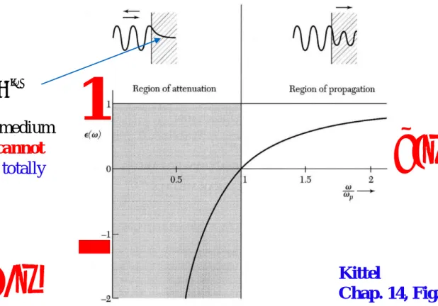
So, what is happening when ω < ω_p?

E=E₀e^i(kz-wt) =E₀e^{i(ik wcz-wt)} =E₀e^{-kwc z}e^-iwt

Decaying or attenuating waves through medium (no propagation). The incoming light cannot penetrate through the medium, and is totally reflected (approximately).

ε(ω) = 1 + 4piσ(ω)/ω

from Maxwell’s Eqs.

A/M Eq. (1.35)

1

-

^Kittel Chap. 14, Fig. 1

ε(ω)

Metal (~ Free Electron Gas)

_

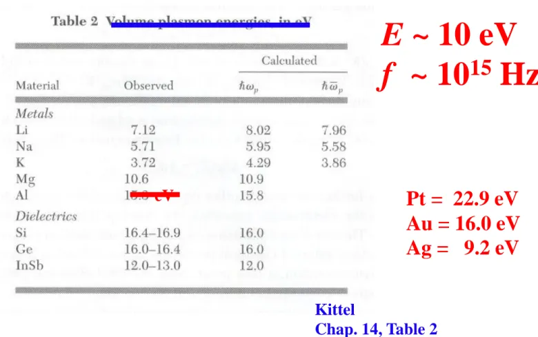
^eV

E ~ 10 eV f ~ 10 15 Hz

Pt = 22.9 eV Au = 16.0 eV Ag = 9.2 eV

____

Kittel

Chap. 14, Table 2

Plasmon Energy (in 3D)

Visible

“Ultraviolet transparency of metals”

This is why metals like silver and aluminium are shiny and have been used for making mirrors for centuries.

Band theory is needed to explain why some metals (e.g. copper and gold) are coloured.

Schematic Figure

Low Energy

w

_p High Energy

ѲE=e₀m₀ ^¶2E

¶t² +m₀s ^¶E

¶t Using E=E₀e^i(k×r-wt)

-k²E₀ = -e₀m₀w^2E₀ -im₀s⁽w⁾w^E₀ k² =e₀m₀w² +im₀s⁽w⁾w = w²

c² 1+ is⁽w⁾ e₀w æ

èç

ö ø÷

Therefore, under AC field, the conductivity becomes a complex number. How does this affect the light propagation? We plug this relation into the Maxwell equation in media.

We have seen in the previous section that the general dispersion relation can be handled conveniently in terms of complex refractive index or dielectric constant.

Therefore,

By defining w_p = ne²

e₀^m : plasma frequency

=1-w²_p w²

w²t² 1+w²t^{2 +i}

w_p² w²

wt 1+w²t²

=e₁⁽w⁾+ie₂⁽w⁾

(Plasma is a medium with equal concentration of positive and negative charges, of which at least Reflections for metals

(skip)

τ in metal is typically on the order of 10 fs or 10^-14 s and the frequency of the visible light is >

10¹⁴ Hz, ωτ = 2πfτ >> 1 and we can neglect the imaginary part:

“Plasma reflectivity”

(skip)

FYI

____________

________

_________ ____

________________________________

_______

E=E₀e^i(kz-wt) =E₀e^{i((n+ik)wcz-wt)} =E₀e^{-kwc z}eⁱ⁽

nw c z-w^t)

Skin Depth

The length over which the current density decays by 1/e in comparison to that at surface is called the

skin depth

(δ). Since J ∝ E,

At low frequencies (ω << 1/τ and ω_p). In this case, ε₂ >> ε₁ and

d = c kw ⁼

c w

2e₀w s₀ ⁼

2 s₀wm₀

_ __

~5 nm in Pt at 4 eV

In materials, there are several sources of

polarization. First, we focus on the polarization by electrons bound to nucleus. This can be well captured by the Lorenz model with certain

resonance frequencies. For simplicity, let’s assume that one electron vibrates.

4B.2. Several Sources of Polarization

md²x

dt² +mg ^dx

dt +mw₀^2x= -eE(t) γ: damping rate Using the complex notation, E(t)= E₀e^-iwt, x(t)= x₀e^-iwt

-mw^2x₀^e-iwt -imgw^x₀^e-iwt +mw₀^2x₀^e-iwt = -eE₀e^-iwt x₀ = -eE₀ /m

w₀²-w² -igw

If the number density of dipoles are N, the polarization P is given by P= -Nex= Ne²

m

1

w₀²-w²-igw ^E0e-iw

t = Ne²

m

1

w₀²-w²-igw ^E(t)

In general

¾¾¾¾®P= Ne² m

1

w₀²-w²-igw ^E

This gives the dielectric susceptibility:

P=e c^E®c = Ne² e

1

w w gw

Now we turn our attention to the polarization in the dielectric medium.

-Thu/11/5/2020 -Final Exam

Tue/12/8/2020

____

i) Electronic Polarization

e_r⁽w⁾=1+c =1+ Ne² e₀^m

1

w₀²-w²-igw e₁⁽w⁾=1+ Ne²

e₀^m

w₀² -w² w₀²-w²

( )

²⁺

( )

^{gw 2, e2(w)= Ne}

2

e₀^m

gw w₀²-w²

( )

²⁺

( )

^{gw 2}

The medium is polarized when ω is lower than ω₀. However, when ω becomes much higher than ω₀, the oscillator does not exhibit any dielectric polarization. This is because the oscillator cannot follow the field change. Consequently, the refractive index steps down as ω crosses ω₀. 1+ Ne² 1

e₀^mw₀²

Energy is lost or absorbed by the medium most strongly at the resonant frequency. This is called the

dielectric loss

. 1

____

i) Electronic Polarization

_ _

~eV

(a) A NaCl chain in the NaCl crystal without an applied field. Average or net dipole moment is zero.

(b) In the presence of an applied field the ions become slightly displaced which leads to a net average dipole moment.

Other Polarization Mechanisms: ii) Ionic Polarization

This corresponds to the optical mode. Therefore, the resonance frequency in the ionic polarization corresponds to the optical frequency (~10 THz) that corresponds to infrared (IR) . Those phonon modes that can respond to IR are called to be IR-active. The lattice absorption by the IR-active phonon modes is specifically called the Reststrahlen (German: residual rays) absorption.

On the other hand, the polarization by the acoustic mode is possible (piezoelectric response), but its magnitude is much smaller than

~THz

(a) A HCl molecule possesses a permanent dipole moment p₀.

(b) In the absence of a field, thermal agitation of the molecules results in zero net average dipole moment per molecule.

(c) A dipole such as HCl placed in a field experiences a torque that tries to rotate it to align p₀ with the field E.

(d) In the presence of an applied field, the dipoles try to rotate to align with the field against thermal agitation. There is now a net average dipole moment per molecule along the field.

Other Polarization Mechanisms: iii) Dipolar Polarization

In materials such as water, the molecules have permanent dipole moments even before the application of external field. However, they are randomly distributed so the average dipole moment (p_av) is equal to zero.

Under the external field, the dipole moment tends to align parallel to the field while the magnitude remains to be same. This results in the finite p_av. The following figure is on the example of HCl liquid.

~GHz

p = 1 3

p

₀²

E

kT = a

_d

E

^p0: permanent dipole moment α_d: polarizability

dp(t )

dt = - p(t ) - a

_d

E(t ) t

p(t + dt ) = p(t ) - dt

t

_d

( p(t ) - a

_d

E

₁

)

dp(t )

dt = - p(t ) - a

_d

E

1

t

_d

In general, for the time-varying AC field of E(t)

1

1

Schematic Figure Only

iii) Dipolar Polarization

E(t)

P(t)

The response of the dipole under AC field can be treated in complex notation as usual:

E(t)= E₀e^-iwt, p(t)= p₀e^-iwt dp(t)

dt = - p(t)-

a

_d^E(t)

t

_d ^{® -i}

w

^p₀ = - p₀ -

a

_d^E₀

t

_d p₀ =

a

_d^E₀

1-i

wt

_d ^\p(t)=

a

_d

1-i

wt

_d ^E(t)

If N is the number density of dipolar molecules,

P = Np(t) = N a

_d

1 - i wt

_d

E, c = N a

_d

e

₀

1 1- i wt

_d

The relaxation time characterizes the resonance frequency in dipolar polarization. The difference is that ε₁(ω) decreases monotonically rather than sharp oscillation as in the Lorentz oscillator.

ε₂(ω)

Schematic Figure Only iii) Dipolar Polarization

~GHz

2.4 GHz for microwave oven

τ_d ~ 100 ps (water) and ~ ms (ice)

Schematic Figure Only iii) Dipolar Polarization

ε 1 ε r ε ′

ε 2 ε i ε ″

(a) A crystal with equal number of mobile positive ions (ex. H+, Li+) and fixed negative ions. In the absence of a field, there is no net separation between all the positive charges and all the negative charges.

(b) In the presence of an applied field, the mobile positive ions migrate toward the negative charges and positive charges in the dielectric. The dielectric therefore exhibits interfacial polarization.

(c) Grain boundaries and interfaces between different materials frequently give rise to Interfacial polarization.

Other Polarization Mechanisms: iv) Interfacial Polarization

The relaxation time for the interfacial polarization is much longer than the dipolar relaxation time. Therefore, the dielectric loss occurs at much lower frequencies.

Schematic Figure

~100 mm

The frequency dependence of the real and imaginary parts of the dielectric constant in the presence of interfacial, dipolar, ionic, and, electronic polarization mechanisms.

Optical dielectric constant (ε^∞) Static dielectric

constant (ε⁰):

f < 10 GHz

ε

₁

ε

₂

__

~THz ~eV

~GHz

~Hz

__ _

__

real

imaginary

ε

₁

ε

_r

ε ′

ε

₂

ε

_i

ε ″

4C. Quantum Phenomena: Absorption

4C.0. Vertical Transition and Photon Absorption 4C.1. Interband Transition: Semiconductor

4C.2. Interband Transition: Metal 4C.3. Exciton

4C.4. Free Carrier Absorption 4C.5. Surface Plasmon

4C.6. Raman Spectroscopy

The classical theory of polarization and conductivity gave good account of light-matter interactions on a macroscopic scale. Nevertheless, fine details are not fully captured by this approach, which requires consideration of quantum effects.

By the quantum effects we mean the band structure for electrons and particle nature for waves (photon for electromagnetic waves and phonon for lattice vibrations). The light-matter interactions are essentially among these three parties. The quantum process explicitly describes how electrons absorb or emit photons, possibly together with absorption or emission of phonons. Therefore, it directly relates to the absorption and emission process within the material. We will first focus on the photon absorption.

Since the photon and phonon are bosons, they can be created or annihilated. In Chap. 3B, we have seen that in the electron-phonon collision, the energy and crystal-momentum conservations should be satisfied in the collision process. The same principle applies to the interaction involving the photon: the energy and momentum should be conserved. (The crystal momentum for electrons or phonons.) For instance, suppose that an electron in (n_i,k_i) absorbs one photon with (ω,k) and occupy a new electron state (n_f,k_f) which should be empty before the transition (due to the Pauli exclusion principle). The related conservation laws are:

This to say, k is so small that

k

_f

is essentially identical to k

_i. This corresponds to the vertical transition as shown in the band diagram.

This is because the light is so light (massless) that it can deliver meaningful momentum. The transition should be between different bands, and so it is interband transition.

As a result, electron-hole pair is created. Note that the transition requires that the final state is empty because of

18 20 22 24 26 28 30

18 20 22 24 26 28 30

Photon ħω = ΔΕ

ΔE

Conservation laws for photon absorption

4C.0. Vertical Transition and Photon Absorption

_______

______ _____

____ ________

The absorption of photon occurs in a probabilistic way (that follows the Fermi golden rule). Suppose that a packet of photons are passing through the medium. After they pass over a certain length, say 1 μm, some percentage of photons are absorbed and lost from the packet. For the next travel over the same length, the same percentage of the remaining photons will be absorbed. In this way, the intensity of light that is equal to the number photons, is reduced exponentially, which is nothing but the Beer’s law.

The absorption coefficient is typically in the range of 10³- 10⁵ cm^-1 for semiconductors. That is to say, for a photon to be absorbed, it should travel at least 100 nm, going past over hundreds of lattice sites and electrons. This means that the absorption probability is rather low.

This also implies that multi-photon absorption process in which several photons are simultaneously absorbed by one electronic transition happens in a much lower chance than single-photon absorption.

In the next sections, we will examine electronic transitions in various situations.

Thicknesses of LED

Solar Cells

Water Splitting

? Multi-Photon Absorption Process by One Electronic Transition ?

4C.1. Interband Transition: Semiconductor

The insulators have an energy gap between occupied and unoccupied states. This means that the photon is not absorbed by electrons with its energy below the energy gap.

For the direct-bandgap material such as GaAs and InAs, the absorption starts right from the bandgap if photon energy ħω is equal to E_g. The absorption creates one electron in the conduction band bottom and one hole in the valence band top.

With higher photon energies, more electron-hole pairs are available for the absorption because DOS increases with the square-root of electron or hole energies. This increases the absorption coefficient as more transitions can happen.

Direct Bandgap

JDOS: why depends only on square root? If the transition can happen over any two states then JDOS should be the square of square-root. However,

__

Free Electron Model (spin-up or spin-down)

𝛼

hν

GaAs Absorption Edge

E g (T)

E g

Free Electron Model

𝛼

hν