Chapter 3.
Gas Liquefaction System
Cryogenic Engineering
KIM, Min Soo
3.1 System Performance Parameters
▪ System performance parameters
• Work required
Unit mass of gas compressed = −Wሶ
ሶm
• Work required
Unit mass of gas liquefied = − Wሶ
ሶ
mf
• Liquefiecd fraction of the total flow of gas = y = −mሶf
ሶm
• Figure of Merit FoM = Theoretical work
Actual work = −Wሶሶi
W (0~1)
▪ Gas – liquefaction systems
The systems that can produce low temperatures required for liquefaction.
+
Additional performance parameters• Compressor adiabatic efficiency
• Expander adiabatic efficiency
• Compressor mechanical efficiency
• Expander mechanical efficiency
• HX effectiveness
• Pressure drop
• Heat transfer to the system
3.1 System Performance Parameters
3.2 Thermodynamically Ideal Cycle (Liquefaction system - open cycle)
P1 P2
T
S
2 1
ሶ f
𝑊𝑐
ሶ𝑄𝑅
ሶ
𝑚
1 2
ሶ𝑊𝑒
𝑓
ሶ
𝑚𝑓
1-2: Isothermal compression
2-f: Isentropic expansion(expander) In this case, P2 = 70 ~ 80 GPa for N2
(too high!)
▪ Apply 1st and 2nd laws of thermodynamics to the system
1st law of thermodynamics:
ሶ𝑄𝑛𝑒𝑡 − ሶ𝑊𝑛𝑒𝑡 =
𝑜𝑢𝑡𝑙𝑒𝑡𝑠
ሶ
𝑚 ℎ + 𝑣2
2𝑔𝑐 + 𝑔𝑧
𝑔𝑐 −
𝑖𝑛𝑙𝑒𝑡𝑠
ሶ
𝑚 ℎ + 𝑣2
2𝑔𝑐 + 𝑔𝑧 𝑔𝑐
→ ሶ𝑄𝑛𝑒𝑡 − ሶ𝑊𝑛𝑒𝑡 =
𝑜𝑢𝑡𝑙𝑒𝑡𝑠
ሶ
𝑚ℎ −
𝑖𝑛𝑙𝑒𝑡𝑠
ሶ
𝑚ℎ
→ ሶ𝑄𝑅 − ሶ𝑊𝑖 = ሶ𝑚(ℎ𝑓−ℎ1) = − ሶ𝑚(ℎ1−ℎ𝑓) (𝑊ሶ𝑖 = 𝑊𝑒 − 𝑊𝑐)
3.2 Thermodynamically Ideal Cycle (Liquefaction system - open cycle)
▪ Apply 1st and 2nd laws of thermodynamics to the system
2ndlaw of thermodynamics:
ds = δqቇ
T rev,ideal
→ δq = T ∙ ds
→ QሶR = ሶmT1 S2 − S1 = − ሶmT1 S1 − Sf
3.2 Thermodynamically Ideal Cycle (Liquefaction system - open cycle)
▪ Apply 1
stand 2
ndlaws of thermodynamics to the system
From 1st and 2ndlaws of thermodynamics,
ሶQR − ሶWi = ሶm(hf−h1) = − ሶm(h1−hf) ⋯ 1st law ሶQR = ሶmT1 S2 − S1 = − ሶmT1 S1 − Sf ⋯ 2nd law
→ −𝐖ሶ 𝐢
ሶ
𝐦 = 𝐓𝟏 𝐒𝟏 − 𝐒𝐟 − 𝐡𝟏 − 𝐡𝐟 = − 𝐖ሶ 𝐢
ሶ
𝐦𝐟
* m = ሶሶ mf → liquid yield 𝐲 = 𝐦ሶ𝐟
ሶ𝐦 = 𝟏
3.2 Thermodynamically Ideal Cycle (Liquefaction system - open cycle)
3.2 Thermodynamically Ideal Cycle (Liquefaction system - open cycle)
3.3 Joule – Thomson Effect (Expansion device – valve)
ሶ𝑄𝑅
ሶ𝑊𝑆
ℎ1 ℎ2
1stlaw of thermodynamics:
ሶQR − ሶWS =
outlets
ሶ
m h + v2
2gc + gz
gc −
inlets
ሶ
m h + v2
2gc + gz gc
→ 0 = ሶm(h2−h1)
→ 𝐡 = 𝐡
▪ Expansion valve
▪ Joule – Thomson coefficient
𝛍𝐉𝐓 = 𝛛𝐓ቇ
𝛛𝐏 𝐡
→ Change in temperature due to a change in pressure at constant enthalpy (Slope of isenthalpic line)
3.3 Joule – Thomson Effect (Expansion device – valve)
▪ Joule – Thomson coefficient
𝛍𝐉𝐓 = 𝛛𝐓ቇ
𝛛𝐏 𝐡
→ Slope of isenthalpic line
Isenthalpic expansion of a real gas.
3.3 Joule – Thomson Effect (Expansion device – valve)
T
P
constant enthalpy
𝑃2←𝑃1 𝑃2’←𝑃1’
P2←P1 : Temperature ↓ if Pressure ↓ → 𝛍𝐉𝐓 > 𝟎 P2′←P1′ : Temperature ↑ if Pressure ↓ → 𝛍𝐉𝐓 < 𝟎
3.3 Joule – Thomson Effect (Expansion device – valve)
▪ Joule – Thomson coefficient
μJT = 𝜕Tቇ
𝜕P h
= −𝜕Tቇ
𝜕h P
𝜕hቇ
𝜕P T
from basic thermodynamics (Van Wylen and Sonntag, 1976),
dh = 𝜕hቇ
𝜕T P
dT + 𝜕hቇ
𝜕P T
dP = CP dT + v − T 𝜕vቇ
𝜕T P
dP
→ 𝜕hቇ
𝜕T P
= CP, 𝜕hቇ
𝜕P T
= v − T 𝜕vቇ
𝜕T P
3.3 Joule – Thomson Effect (Expansion device – valve)
▪ Joule – Thomson coefficient
μJT = 𝜕Tቇ
𝜕P h
= −𝜕Tቇ
𝜕h P
𝜕hቇ
𝜕P T
= 1
CP T 𝜕vቇ
𝜕T P
− v
For an ideal gas,
𝜕vቇ
𝜕T P
= R
P = v T
μJT = 1
CP T 𝜕vቇ
𝜕T P
− v = 0
3.3 Joule – Thomson Effect (Expansion device – valve)
▪ Joule – Thomson coefficient
μJT = 1
CP T 𝜕vቇ
𝜕T P
− v = − 1
CP 𝜕uቇ
𝜕P T
+ 𝜕(Pv)
𝜕P T
from h = u + Pv,
Variation of the product 𝑃𝑣
with pressure and temperature for a real gas.
3.3 Joule – Thomson Effect (Expansion device – valve)
▪ Van der Waals gas
P + a
v2 v − b = RT
Equation of state (EOS)
▪ Joule – Thomson coefficient for van der Waals gas
μJT = 2a/RT 1 − b/v 2 − b CP 1 − 2a
vRT 1 − b v
2
μJT = 1 CP
2a RT − b
for large value of the specific volume,
3.3 Joule – Thomson Effect (Expansion device – valve)
▪ Inversion curve for van der Waals gas
μJT = 2a/RT 1 − b/v 2 − b CP 1 − 2a
vRT 1 − b v
2 = 0 → 2a/RT 1 − b/v 2 − b = 0
The inversion curve is represented by all points at which the Joule-Thomson coefficient is zero.
Ti = 2a
bR 1 − b v
2
▪ Inversion temperature for van der Waals gas
3.3 Joule – Thomson Effect (Expansion device – valve)
Ti = 2a
bR 1 − b v
2
Ti,max = 2a
bR < Troom ∶ He, H2, Ne
→ Cannot produce low T with expansion valve alone.
(Require expander, turbine)
3.3 Joule – Thomson Effect (Expansion device – valve)
3.4 Adiabatic Expansion
T
s P
HP
LS (Isentropic)
H (Isenthalpic) T (Isothermal)
▪ Work producing device : expansion engine (turbine)
Adiabatic Expansion : Most effective means of lowering T of the gas
(※ Adiabatic + Reversible = Isentropic!)
Problem : 2 Phase Mixture in an expander!
▪ Isentropic expansion coefficient, μs
μs = 𝜕T
𝜕𝑃 𝑠
= − 𝜕𝑇
𝜕𝑠 𝑝
𝜕𝑠
𝜕𝑃 𝑇
= 𝑇 𝐶𝑝
𝜕𝑣
𝜕𝑇 𝑃
CP = 𝜕h
𝜕T P
= 𝜕Q
𝜕T p
, Q = TdS
Maxwell’s Relation −
𝜕𝑆𝜕𝑃 𝑇
= (
𝜕𝑉𝜕𝑇
)
𝑃3.4 Adiabatic Expansion
▪ Isentropic expansion coefficient, 𝜇𝑠
μs = 𝜕T
𝜕P s
= − 𝜕T
𝜕s p
𝜕s
𝜕P T
= T Cp
𝜕v
𝜕T P
Volume expansion coefficient β = 1 v
𝜕v
𝜕T P
= v Cp
For Ideal gas : 𝜕v
𝜕T P
= R P = v
T
= T Cp βv
Pv = RT
For Van der Waals gas :
(P + a
v2)(v − b) = RT
= v(1 −b
v) Cp[1 − 2a
vRT 1 − b v
2
]
3.4 Adiabatic Expansion
- External work method :
energy is removed as external work
- Internal work method (Expansion Valve) : do not remove energy from gas
but moves molecules farther apart
▪ Methods of cooling
3.4 Adiabatic Expansion
Liquefaction Systems for Gases
3.5 Linde-Hampson
3.6 Precooled Linde 3.8 Cascade 3.13 LNG (Cascade)
3.7 Linde dual-P 3.12 Claude dual-P
3.9 Claude 3.10 Kapitza 3.11 Heylandt
( For Ne, H2, He ) 3.15 Linde 3.16 Claude 3.17 He system 3.19 Collins He system
3.14 Comparison of Liquefaction Systems
3.18 Ortho-para H2 Conversion
= A big purpose for learning cryogenic systems!
(Korea’s energy supply is heavily dependent on import by ships!)
T
P
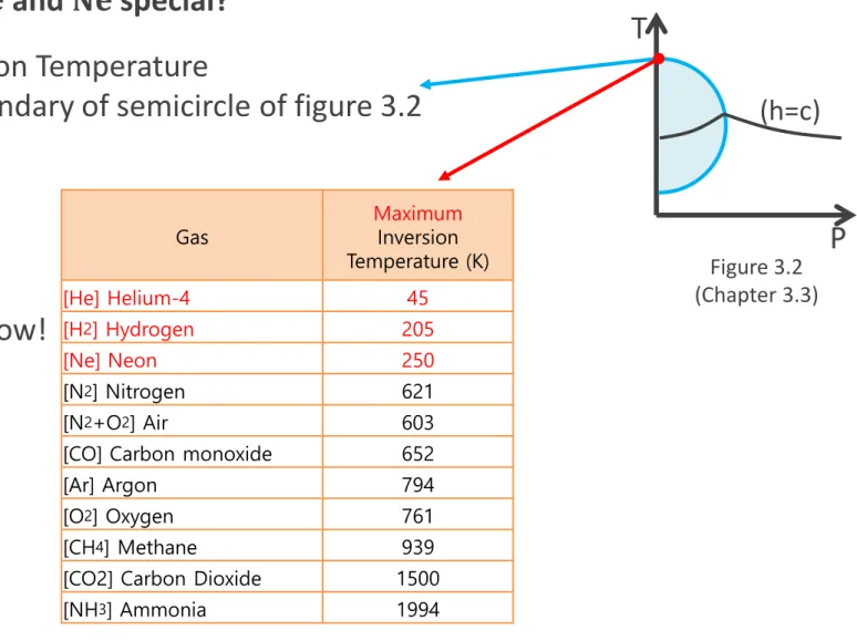
(h=c)
Figure 3.2 (Chapter 3.3)
Gas Maximum
Inversion Temperature (K)
[He] Helium-4 45
[H2] Hydrogen 205
[Ne] Neon 250
[N2] Nitrogen 621
[N2+O2] Air 603
[CO] Carbon monoxide 652
[Ar] Argon 794
[O2] Oxygen 761
[CH4] Methane 939
[CO2] Carbon Dioxide 1500
[NH3] Ammonia 1994
Inversion Temperature
= boundary of semicircle of figure 3.2 Why are 𝐇𝟐, 𝐇𝐞 and 𝐍𝐞 special?
Very Low!
3.4 Adiabatic Expansion
In semicircle, μJT > 0
= Isenthalpic expansion (J-T Valve) is cooling!
Out of semicircle, μJT < 0
= Isenthalpic expansion (J-T valve) is heating!
= We cannot make liquid by J-T valve!
= To make liquid, we must applicate expander or dual- pressure or pre-cooling.
T
P
Case of H2, He, Ne (Circle is very small)
Why are 𝐇𝟐, 𝐇𝐞 and 𝐍𝐞 special?
(h=c) (-)
3.4 Adiabatic Expansion
3.5 Simple Linde-Hampson System
The most simple gas liquefaction/separation system.
This system is based on the Joule-Thomson effect.
Chapter 3.3. When a (non-ideal) gas expands, it will cold down (below inversion temperature). This is why our whistle is colder than our body temperature!
William Hampson and Carl von Linde independently filed for patent
of the cycle in 1895.
▪ History
3.5 Simple Linde-Hampson System
Enhance from Siemens cycle(1857) to Linde-Hampson cycle(1895)
A : Compression B : Cooling
C : Cooling (HX) D : Expansion C : Heating (HX)
A : Compression B : Cooling
C : Cooling (HX)
D : Joule-Thompson Orifice
(Reservoir + Expansion Valve) C : Heating (HX)
▪ History Brother founds He founds himself
3.5 Simple Linde-Hampson System
Siemens cycle has poor efficiency and is only efficient for high temperature gases. But Linde-Hampson cycle can easily collect liquid and cool
dramatically.
Heike Kamerlingh Onnes made ‘liquid helium’ (1908)
by this Linde-Hampson system and found ‘super-conductivity’.
And He got Nobel prize in Physics (1913)!
▪ History
3.5 Simple Linde-Hampson System
▪ Diagram
Control Volume
3.5 Simple Linde-Hampson System
T
s P
H② ①
③
④
ⓕ ⓖ
P
Lh
T
Normal room : T1=300K, P1=1bar Liquid N2 : T4=77K
Constant T : Isothermal Constant P : Isobaric Constant h : Isenthalpic
▪ Diagram
3.5 Simple Linde-Hampson System
Another form of diagrams
Control Volume
Control Volume
▪ Diagram
3.5 Simple Linde-Hampson System
Quality x = (mass of sat. gas) (total mass)
(※ Volume of gas is very larger than liquid)
Assumption
- Reversible pressure drop - No heat in-leak
(Reversible isothermal process in compressor) - 100% effective heat exchanger
▪ Diagram
3.5 Simple Linde-Hampson System
Liquid yield y = mf
m = h1 − h2 h1 − hf
At control volume, mhሶ 2 = m − ሶሶ mf h1 + ሶmhf Q1. We can choose P2 in the system. Which is best P2?
① CV
② ⓕ
▪ Questions
3.5 Simple Linde-Hampson System
Best P2 is 𝜕y
𝜕P2 = 0
𝜕h2
𝜕P2 = 0
(h1, hf is fixed value)
𝜕h
𝜕P = −μJTCP
(CP is positive number) μJT = 0
μJT is slope at T-P diagram.
So, semicircle in T-P graph means best P2! (Inversion Curve) (Chapter 3.3)
T
P
(+) (-) (0)
▪ Questions
3.5 Simple Linde-Hampson System
Q2. How much works do we need for running this system?
ሶQR − ሶW = ሶm(h2 − h1)
At compressor,
−Wሶ
ሶ
m = T1(s1 − s2) − (h1 − h2)
※ QRሶ = ሶmT1(s1 − s2)
− Wሶ
ሶ
mf = − Wሶ
ሶ
my = (h1 − hf
h1 − h2)[T1 s1 − s2 − h1 − h2 ]
▪ Questions
3.5 Simple Linde-Hampson System
Q3. What will happen in real system without assumption?
Reversible pressure drop
→ P2 will be lower.
No heat in-leak
Reversible isothermal process in compressor
→ Qelec will be added. And y will be lower.
ሶ
mh2 + Qelec = m − ሶሶ mf h1 + ሶmhf
▪ Questions
3.5 Simple Linde-Hampson System
100% effective heat exchanger
→ Temperature difference at both side will be lower.
To keep temperature difference, we need input more pump work.
(To enlarge mass flow rate)
100℃ 0℃
0℃
40℃ 100℃ 50℃
0℃
20℃
η = 100% η = 50%
▪ Questions
3.5 Simple Linde-Hampson System
▪ It’s not for Ne/H2/He !
T
s P
H② ①
h
P
L③
Reason 1.
Maximum inversion temp. << room temp.
→ Their expansion = heating!
→ Gas in HX warmed rather than cooled!
T
Gas M.I.T. (K) [He] Helium-4 45 [H2] Hydrogen 205
[Ne] Neon 250
X
Figure 3.6
We will learn later… (Chapter 3.15~3.19)
3.5 Simple Linde-Hampson System
T
s P
H② ①
P
LReason 2.
Liquid yield(y) is negative. (h1 < h2)
→ Even if we could attain low
temperature, no gas would be liquefied.
T
y =mf
m = h1 − h2 h1 − hf
③
h
④ XFigure 3.7
▪ It’s not for Ne/H2/He ! We will learn later… (Chapter 3.15~3.19)
3.6 Precooled Linde-Hampson System
Liquid yield versus compressor temperature for a Linde-Hampson system
using nitrogen as the working fluid
• It is apparent that the performance of a Linde-Hampson system could be improved if the gas entered the heat exchanger at a temperature lower than ambient temperature
Precooled Linde-Hampson system
3.6 Precooled Linde-Hampson System
Precooled Linde-Hampson system T-S diagram
3.6 Precooled Linde-Hampson System
▪ Liquid yield
Applying the First Law for steady flow to the heat exchanger, the two liquid receivers, and the two expansion valves.
𝑟 is the refrigerant mass flow rate ratio
ሶ
𝑚𝑟 is the mass flow rate of the auxiliary refrigerant
ሶ
𝑚 is the total mass flow rate through the high pressure compressor
r = m / mr
( )
2 r d f 1 r a f f
mh +m h = m m h− +m h +m h
a d
f 1 2
1 f 1 f
h h
m h h
y r
m h h h h
−
= = − +
− −
3.6 Precooled Linde-Hampson System
The second term of liquid yield represents the improvement in liquid yield that is obtained through the use of precooling.
a d
f 1 2
1 f 1 f
h h
m h h
y r
m h h h h
−
= = − +
− −
▪ Liquid yield
3.6 Precooled Linde-Hampson System
▪ Limit of the liquid yield 1
From the Second Law of Thermodynamics, 𝑇3 and 𝑇6 cannot be lower than the boiling point of the auxiliary refrigerant at point d
3.6 Precooled Linde-Hampson System
▪ Limit of the liquid yield 1 : The maximum liquid yield
With a suitable value of the refrigerant flow-rate ratio r, liquid yield could have a value of 1, which means 100 percent for the liquid yield.
6 3
max
6 f
h h
y h h
= −
−
3.6 Precooled Linde-Hampson System
▪ Limit of the liquid yield 1 : The maximum liquid yield
ℎ3 and ℎ6 are taken at the temperature of the boiling refrigerant at point d)
6 3
max
6 f
h h
y h h
= −
−
Precooled Linde-Hampson cycle
3.6 Precooled Linde-Hampson System
▪ Limit of the liquid yield 2
If the refrigerant flow rate ratio were too large, the liquid at point d would not be completely vaporized, and liquid would enter the refrigerant compressor.
Liquid yield versus refrigerant flow rate ratio for the precooled Linde-Hampson system
using nitrogen as the working fluid
3.6 Precooled Linde-Hampson System
▪ The work requirement
• If the main compressor is reversible and isothermal and the auxiliary compressor is reversible and adiabatic.
• The last term represents the additional work requirement for the auxiliary compressor. (usually on the order of 10 percent of the total work)
( ) ( ) ( )
1 1 2 1 2 b a
W T s s h h r h h
− m = − − − + −
3.6 Precooled Linde-Hampson System
The increase in liquid yield more than offsets the additional work requirement, however, so that the work requirement per unit mass of gas liquefied is actually less for the precooled system than for the simple system.
Work required to liquefy a unit mass of nitrogen in a precooled Linde-Hampson system
▪ The work requirement
3.6 Precooled Linde-Hampson System
3.7 Linde Dual-Pressure Cycle
Linde dual-pressure system
3.7 Collins Helium-Liquefaction System
Linde dual-pressure system T-S diagram
3.7 Linde Dual-Pressure Cycle
▪ Liquid yield
Applying the First Law for steady flow to the heat exchanger, the two liquid receivers, and the two expansion valves.
𝑖 is the intermediate pressure stream flow rate ratio
ሶ
𝑚𝑖 is the mass flow rate of the intermediate pressure stream at point 8
ሶ
𝑚is the total mass flow rate through the high pressure compressor
( )
3 f f i 2 i f 1
mh =m h +m h + m m− −m h
1 3
f 1 2
1 f 1 f
h - h
m h - h
y i
m h - h h - h
= = −
i = m / mi
▪ Liquid yield
• This modification reduces the liquid yield somewhat.
• The second term of liquid yield represents the reduction in the liquid yield below that of the simple system because of splitting the flow at the intermediate pressure liquid receiver.
1 3
f 1 2
1 f 1 f
h - h
m h - h
y i
m h - h h - h
= = −
3.7 Linde Dual-Pressure Cycle
Applying the First Law for steady flow to the two compressors.
(
QR1 −WC1) (
+ QR 2 −WC2)
= mh3 −(
m−m hi)
1 −m hi 2( ) ( )
( )
R1 i 1 1 2
R 2 1 2 3
Q m m T s s
Q mT s s
= − − −
= − −
( ) ( ) ( ) ( )
1 1 3 1 3 1 1 2 1 2
W T s s h h i T s s h h
m
− = − − − − − − −
▪ The work requirement
3.7 Linde Dual-Pressure Cycle
3.7 Linde Dual-Pressure Cycle
▪ The work requirement
This modification reduces the total work required.
The work requirement is reduced below that of the simple system by the amount given by the second bracketed term.
( ) ( ) ( ) ( )
1 1 3 1 3 1 1 2 1 2
W T s s h h i T s s h h
m
− = − − − − − − −
Work required to liquefy a unit mass of air in the Linde dual-pressure system
3.7 Linde Dual-Pressure Cycle
▪ Optimal intermediate pressure
• As ‘Work required to liquefy a unit mass of air in the Linde dual-
pressure system’ shows, there is an optimum intermediate pressure p2 for a given intermediate stream mass flow rate ratio, which makes the work requirements a minimum.
• Typical air liquefaction plants operate with i = 0.8, p3= 200atm, p2 between 40 and 50 atm.
3.7 Linde Dual-Pressure Cycle
3.8 Cascade System
• The cascade system is an extension of the precooled system
• There are refrigeration system chain of ammonia – ethylene – methane -nitrogen
• From a thermodynamic point of view, the cascade system in very desirable for
liquefaction because it approaches the ideal reversible system more closely than any other discussed thus far0
ሶ
mfhf + m − ሶሶ mf h1 − ሶmh2 +
i=1 ncomp
ሶ
mx,i ha,i − hb,i + ሶmx,n hb,n − hc,n = 0
y = h1 − h2
h1 − hf +
i=1 n_comp
xihi,i − he,i
h1 − hf + ሶmx,n hb,n − hc,n
− ሶW = ሶm[ h2 − h1 − T1 h2 − h1 ]hf +
i=1 n_comp
ሶ
mx,i he,i − hi,i
−Wሶ
ሶ
m = [ h2 − h1 − T1 h2 − h1 ]hf +
i=1 n_comp
xi he,i − hi,i
Liquid yield :
Power per mass flow :
3.8 Cascade System
Cryogenic System Video
Cryogenic System Video
Cryogenic System Video
3.9 Claude System
In 1902 Claude devised what is now known as the Claude system for liquefying air. The system enabled the production of
industrial quantities of liquid nitrogen, oxygen, and argon
Georges Claude(1870-1960)
3.9 Claude System
Claude system
3.9 Claude System
Claude system T-S diagram
3.9 Claude System
▪ Valve VS Expansion engine or expander
• The expansion through an expansion valve is an irreversible process.
Thus if we wish to approach closer to the ideal performance, we must seek a better process.
• If the expansion engine is reversible and adiabatic, the expansion
process in isentropic, and a much lower temperature is attained than an isenthalpic expansion.
3.9 Claude System
▪ Why we can not eliminate the expansion valve?
The expansion valve could not be eliminated because of the problem of two-phase flow within the engine cylinder or turbine blade flow passages.
3.9 Claude System
▪ Liquid yield
Applying the First Law for steady flow to the heat exchangers, the expansion valve, and the liquid receiver as a unit, for no external heat transfer.
x is the fraction of the total flow that passes through the expander
ሶ
𝑚𝑒 is the mass flow rate of fluid through expander
ሶ
𝑚is the total mass flow rate through the high pressure compressor
x =m / me
( )
2 e e f 1 e 3 f f
mh +m h = m m h− +m h +m h
3 e
f 1 2
1 f 1 f
h h
m h h
y x
m h h h h
−
= = − +
− −
3.9 Claude System
▪ Liquid yield
The second term of liquid yield represents the improvement in performance over the simple Linde Hampson system.
3 e
f 1 2
1 f 1 f
h h
m h h
y x
m h h h h
−
= = − +
− −
3.9 Claude System
▪ The work requirement
( ) ( )
1 1 2 1 2
W T s s h h
− m = − − −
The work requirement per unit mass compressed is exactly the same as that for the Linde Hampson system if the expander work is not utilized to help in the compression.
The work requirement per unit mass compressed for the Linde Hampson system
3.9 Claude System
c e
W W
W
m m m
− = − −
If the expander work is used to aid in compression, then the net work requirement is given by
( )
e
3 e
W x h h
m = −
( ) ( )
c
2 1 1 1 2
W h h T s s
m = − + −
The net work is given by
( ) ( ) ( )
1 1 2 1 2 3 e
W T s s h h x h h
m
− = − − − − −
▪ The work requirement
3.9 Claude System
▪ The work requirement
The last term is the reduction in energy requirements due to the utilization of the expander work output.
( ) ( ) ( )
1 1 2 1 2 3 e
W T s s h h x h h
m
− = − − − − −
3.9 Claude System
Work required to liquefy a unit mass of air in the Claude system
3.9 Claude System
▪ Smallest work requirement per unit mass liquefied
• There is a finite temperature at point 3 that will yield the smallest work requirement per unit mass liquefied.
• As the high pressure is increased, the minimum work requirement per unit mass liquefied decreases.
3.10 Kapitza System
• Modified Claude system which
eliminate the third low temperature heat exchanger
• A rotary expansion engine was used instead of a reciprocating expander
• Kapitza system usually operated at relatively low pressures-on the order of 700kPa
3.10 Kapitza System
ሶ
mfhf + m − ሶሶ mf h1 − ሶmh2 + ሶmx h3 − he = 0
y = h1 − h2
h1 − hf + xh3 − he h1 − hf
− ሶW = ሶm[ h2 − h1 − T1 h2 − h1 ]hf + ሶmx he − h3
−Wሶ
ሶ
m = [ h2 − h1 − T1 h2 − h1 ]hf + x he − h3
Liquid yield :
Power per mass flow :
3.11 Heylandt System
(Claude system has one more HX at here)
3.11 Heylandt System
For a high pressure (Approximately 20 MPa ≒ 200 atm)
For an expansion-engine (flow-rate ratio of approximately 0.6) The optimum value of T before expansion = near ambient T
→ So, it can eliminate first HX in the Claude system by compressing!
(∴ Modified Claude system) Advantage
→ The lubrication problems in the expander are easy to solve!
(Because T of expander is very low)
※ Contribution of expander and expansion valve is nearly equal.
(At original Claude system, expander makes more contribution)
3.12 Other Liquefaction Systems Using Expanders
Dual-pressure Claude System Linde Dual-pressure (Chapter 3.7)
3.12 Other Liquefaction Systems Using Expanders
… It is similar to the Linde dual-pressure system. (Chapter 3.7) (A reservoir is replaced by expander and two HX)
Advantage
Gas through expander is compressed to some intermediate P.
→ Work requirement per unit mass of gas liqefied is reduced.
※ If nitrogen compressed from 1 atm to 35 atm, optimum performance is attained when 75 percent of flow diverted through the expander.
3.13 Liquefaction Systems for LNG
3.13 Liquefaction Systems for LNG
World LNG supply chains
Nord stream
▪ LNG liquefaction
Typical 4 Natural Gases
3.13 Liquefaction Systems for LNG
• Condense at different temperature levels.
• LNG deposits are normally found deeper position than oil
• Deepest deposits can be made of pure LNG
•
The Linde-Hampson system is desirable for small-scale liquefaction plants.
However, the basic Linde-Hampson system with no precooling would not work for neon, hydrogen, or helium
Because the maximum inversion temperature for these gases is below ambient temperature. So, it is normally using for air separation
3.15 Precooled Linde-Hampson System
3.15 Precooled Linde-Hampson System
2 1 1 f
c a c a
h h h h
z y
h h h h
− −
= +
− −
N2
z m
= m
2 2
N N
f f
m m / m z
m = m / m = y
The nitrogen boil-off rate per unit mass of hydrogen or neon compressed
3.15 Precooled Linde-Hampson System
Nitrogen boil-off per unit mass of hydrogen produced for the
liquid-nitrogen-precooled Linde- Hampson system as a function of the liquid-nitrogen bath
temperature.
3.15 Precooled Linde-Hampson System
Liquid hydrogen storage tank system, horizontal mounted with double gasket and dual seal
3.15 Precooled Linde-Hampson System
A complete survey plot of hydrogen storage in metal hydrides and carbon-based materials
3.15 Precooled Linde-Hampson System
3.16 Claude System for Hydrogen or Neon
3.17 Helium-Refrigerated Hydrogen-Liquefaction System
Helium-refrigerated hydrogen liquefaction system
• Relatively low pressures can be used
• The compressor size can be reduced
(although two compressors are required)
• The pipe thickness can be reduced
• The hydrogen or neon need be compressed only to a pressure high enough to overcome the irreversible pressure drops through the heat exchangers and piping in an actual system
▪ Advantage
3.17 Helium-Refrigerated Hydrogen-Liquefaction System
3.18 Ortho-Para-Hydrogen Conversion in the Liquefier
N.B.P. = 20.3K
ortho − H2
(Spins aligned, high energy)
para − H2
(Spins aligned, high energy)
Types of hydrogen molecules
ortho − H2 → para − H2 + Δα (heat of conversion) 70.3 kJ/kg
Latent heat 44.3 kJ/kg
At high temperature is a mixture of 75% 𝑜𝑟𝑡ℎ𝑜 − H2 and 25% 𝑝𝑎𝑟𝑎 − H2 As temperature is cooled to the normal boiling point of hydrogen, the
𝑜𝑟𝑡ℎ𝑜 − H2 concentration decreases from 75 to 0.2%
3.18 Ortho-Para-Hydrogen Conversion in the Liquefier
The changeover from 𝑜𝑟𝑡ℎ𝑜 − to 𝑝𝑎𝑟𝑎 − ℎ𝑦𝑑𝑟𝑜𝑔𝑒𝑛 involves a heat of conversion that is greater than the heat of vaporization of 𝑝𝑎𝑟𝑎 − ℎ𝑦𝑑𝑟𝑜𝑔𝑒𝑛
Therefore serious boil-off losses will result unless measures are taken to prevent it.
3.18 Ortho-Para-Hydrogen Conversion in the Liquefier
3.18 Ortho-Para-Hydrogen Conversion in the Liquefier
▪ Catalysts
hydrous ferric oxide Nickel-based catalyst
3.18 Ortho-Para-Hydrogen Conversion in the Liquefier
▪ Catalysts
Chromic oxide
3.18 Ortho-Para-Hydrogen Conversion in the Liquefier
Helium refrigerator-liquefier at MIT
Samuel C. Collins (MIT) designed Helium liquefier (1952)
It is an extension of the Claude system
3.19 Collins Helium-Liquefaction System
3.19 Collins Helium-Liquefaction System
Collins helium-liquefaction system T-S diagram
3.19 Collins Helium-Liquefaction System
▪ Liquid yield
Consisting of all components except the helium compressor and the expansion engines
y = h1 − h2
h1 − hf + x1 ∆hei
h1 − hf + x2 ∆he2 h1 − hf
x1 = ሶme1/ ሶm x2 = ሶme2/ ሶm
∆hei= enthalpy change of fluid passing through expander 1
∆he2= enthalpy change of fluid passing through expander 2
ሶ
me1, ሶme2 = mass flow rates of fluid through expander 1 and 2, respectively
3.19 Collins Helium-Liquefaction System
▪ Liquid yield
For more than two engines?
→ Additional term similar to the second term for each expander would be added!
3.19 Collins Helium-Liquefaction System
▪ Increase the Collins liquefier performance?
• By using liquid-nitrogen precooling bath
→ Cool-down time would be reduced from 4h to 2h
→ Liquid yield can be tripled
But,
Pre coolant bath is not required because it doesn’t dependent solely on the Joule-Thomson effect!
3.19 Collins Helium-Liquefaction System
3.20 Simon Helium-Liquefaction System
• Liquefy small quantities of helium
• Not operate as a steady-flow system
• It produces helium in a batch process
▪ System Characteristics
3.20 Simon Helium-Liquefaction System
Simon helium-liquefaction system T-S diagram
3.20 Simon Helium-Liquefaction System
▪ Simon helium-liquefaction system process
Process 1-2 : Helium gas is introduced into the heavy-wall container.
(Pressure : 10~15 MPa, Ambient temperature)
Process 2-3 : • Liquid Nitrogen is introduced into the enclosing bath.
• Cools the entire container and contents (77K)
• Vacuum space is filled with helium gas.
(act as heat transfer medium)
• At the completion of the process, inner vessel is thermally isolated
3.20 Simon Helium-Liquefaction System
▪ Simon helium-liquefaction system process
Process 3-4 : Liquid hydrogen is introduced into the upper part of the inner container. Inner container and contents are further cooled to liquid-hydrogen temperature. (20.4 K)
Process 4-5 : • The pressure above the liquid hydrogen is reduced to approximately 0.23 kPa.
• Liquid hydrogen boils as the pressure is lowered until the hydrogen solidifies.
• At the end of the process, the solid hydrogen is at approximately 10 K.
3.20 Simon Helium-Liquefaction System
▪ Simon helium-liquefaction system process
Process 5-6 : • The pressure of the gaseous helium is reduced to atmosphere pressure by allowing the helium to be released to a gas holder external to the system.
• The helium that finally remains in the inner container does work against the helium gas that is discharged.
• The discharged gas removes energy from the system, thereby lowering the temperature of the remaining helium.
• At the end of this process, 75~100% is liquid helium.
3.20 Simon Helium-Liquefaction System
If heat is transferred reversibly, dQ = mcTcdsc = mcccdTc
mc = mass of container Tc = container temperature
cc = container specific heat
3.20 Simon Helium-Liquefaction System
Substituting the Debye expression for the container specific heat, dsc = 233.78RcTc2 dTc
θD3 Integration,
∆sc= −77.93Rc
θD3 (T53 − Tf3)
There is no external heat transfer from the surroundings to the inner vessel,
m
6− m
5s
5− 0 = m
6s
6− m
5s
5