저작자표시

(1)

저작자표시-비영리-변경금지 2.0 대한민국 이용자는 아래의 조건을 따르는 경우에 한하여 자유롭게

l 이 저작물을 복제, 배포, 전송, 전시, 공연 및 방송할 수 있습니다. 다음과 같은 조건을 따라야 합니다:

l 귀하는, 이 저작물의 재이용이나 배포의 경우, 이 저작물에 적용된 이용허락조건 을 명확하게 나타내어야 합니다.

저작권법에 따른 이용자의 권리는 위의 내용에 의하여 영향을 받지 않습니다. 이것은 이용허락규약(Legal Code)을 이해하기 쉽게 요약한 것입니다.

Disclaimer

저작자표시. 귀하는 원저작자를 표시하여야 합니다.

비영리. 귀하는 이 저작물을 영리 목적으로 이용할 수 없습니다.

변경금지. 귀하는 이 저작물을 개작, 변형 또는 가공할 수 없습니다.

(2)

HIGH-PERFORMANCE CONTROL OF IPMSM BY USING MODIFIED-DTC ALGORITHM AND

ANN BASED SPEED CONTROLLER

FOR THE DEGREE OF MASTER PHILOSOPHY

BY

JIA ZHENYU

School of Electrical Engineering

Graduate School of the University of Ulsan May, 2018

[UCI]I804:48009-200000109274 [UCI]I804:48009-200000109274

(3)

HIGH-PERFORMANCE CONTROL OF IPMSM BY USING MODIFIED-DTC ALGORITHM AND

ANN BASED SPEED CONTROLLER

A THESIS SUBMITTED

FOR THE DEGREE OF MASTER PHILOSOPHY

BY

JIA ZHENYU

UNDER THE SUPERVISION OF Prof. Byeongwoo Kim

School of Electrical Engineering

Graduate School of the University of Ulsan

May, 2018

(4)

HIGH-PERFORMANCE CONTROL OF IPMSM BY USING MODIFIED-DTC ALGORITHM AND

ANN BASED SPEED CONTROLLER

Approved by:

Prof.

School of Electrical Engineering (Signature) University of Ulsan

Prof.

School of Electrical Engineering (Signature) University of Ulsan

PhD.

Korea Automotive Technology Institute (Signature)

Date Approved: May, 2018

(5)

ACKNOWLEDGMENTS

During the master course，I experienced and learned a lot of things. I would like to thank many people who have contributed to my research work of this thesis and life in University of Ulsan.

I express my sincere gratitude towards my advisor Professor Byeongwoo, Kim. He is kind and patient all the time. His trust, care and encouragement throughout the past years helped me to insist on researching and solving problems. It is very hard for me to do research work at the beginning, but now I feel honorable for being here. Without his support and patience, my research work and the completion of this thesis would have never become possible.

I would also like to give my heartfelt thanks to the professor Heejun Kang and Hansil, Kim.

They are nice and trusted professors. What’s more, they gave me the opportunity to develop my knowledge of robot control and linear system control, which are important and helpful for me to study servo system control.

Moreover, I give my thankfulness to professor Kanghyun, Jo. In his lectures, I improved my academic English skills and started to know and learn artificial intelligence technique, which is hot popular and very powerful subject. Through his lectures, I also learned about image detection theory, which is important for autonomous vehicle development.

I thank all my colleagues of Automotive Electronics & Control Laboratory, they helped me in my daily lab life and gave me guidance of living in South Korea. Lin Ming helped me a lot in language translation and information delivering. Jungeun Lee is always helpful to me when I have troubles in lab life, I appreciate it deeply. I am grateful to my friend, Wang He, for his helps in paper writing skills.

Last but not the least, I acknowledge the grace of almighty Jesus who leads me at any time and everywhere, Soli Deo Gloria. I sincerely thank my family for the supports and encouragements.

This research was supported by the Industry Core Technology Development Project

"Development of 2kw kg/ ,100kwclass IPMSM electric drive system with high efficiency cooling"

(6)

SUMMARY

HIGH-PERFORMANCE CONTROL OF IPMSM BY USING MODIFIED-DTC ALGORITHM AND ANN BASED SPEED

CONTROLLER

Zhenyu Jia School of Electrical Engineering

The Graduate School University of Ulsan

In this thesis, we present a performance enhancement on direct torque control (DTC) for interior permanent magnet synchronous motor (IPMSM) drive. To solve some key drawbacks of the conventional DTC and space vector modulation (SVM) based DTC control strategies, the predictive controller with super-twist sliding mode (STSM) based torque controller is applied to modify SVM based DTC and backpropagation algorithm based neural network is adopted to tune the parameters of speed controller.

First, a novel STSM torque controller based predictive calculator for generating reference voltage vector is analysed and designed in Chapter 2. This modified DTC strategy is named as STSM-DTC in this thesis. In previous research [27], the classical proportional-integral (PI) torque controller is applied and named as PI-DTC method. In this thesis, both STSM-DTC and PI-DTC strategies combine SVM scheme applied to IPMSM drive. Generally, the torque-ripple and flux-ripple reduction performance has been improved considerably by adopting SVM. The simulation results demonstrate that the proposed STSM-DTC method can enhance the torque control performance furtherly more compared to PI-DTC with smaller torque ripple. Moreover, it has the merits of fast dynamic response, robustness

(7)

against load torque disturbance and speed-ripple reduction, as verified in Chapter 4. In addition, the whole proposed STSM-DTC control strategy, for IPMSM drives can obtain good performance of stator current with very low THD (total harmonic distortion) level.

Next, a novel PI speed controller applying backpropagation based neural network is designed and proposed in Chapter 3. This speed controller is named as NN-PI speed controller in this thesis. The proposed method can overcome the disadvantages of conventional PI controller with high dependence on controlled model and time-consuming parameters-tuning work. Compared to classical PI speed controller, the simulation results prove the effectiveness of the proposed NN-PI speed controller with faster dynamic response, good speed tracking, much smaller speed overshoot and better robustness against load torque variation and load inertia variation, as presented in Chapter 4.

(8)

LIST OF FIGURES

Fig. 1. Block diagram of the conventional DTC for PMSM 7

Fig. 2. Relationship between different quantities in different reference frames 8

Fig. 3. Space voltage vectors and application to control stator flux space vector and torque 9

Fig. 4. Typical topology of three-phase VSI for PMSM 10

Fig. 5. Signal flow chart of generating reference flux vector [27] 12

Fig. 6. Reference voltage vector as a combination of adjacent vectors at sector I 13

Fig. 7. The schematic of proposed STSM torque controller 15

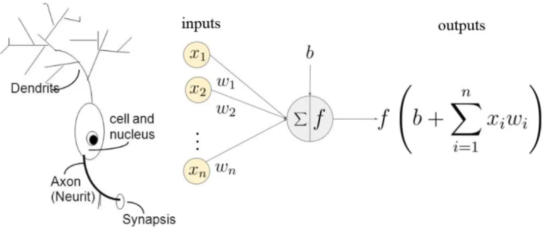
Fig. 8. Biological neuron (left) and artificial neuron (right) 16

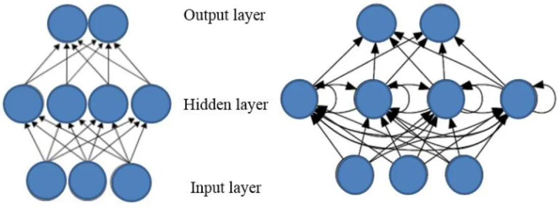
Fig. 9. The topology schematic of three-layered FNN (left) and RNN (right) 17

Fig. 10. The structure of BP neural network 18

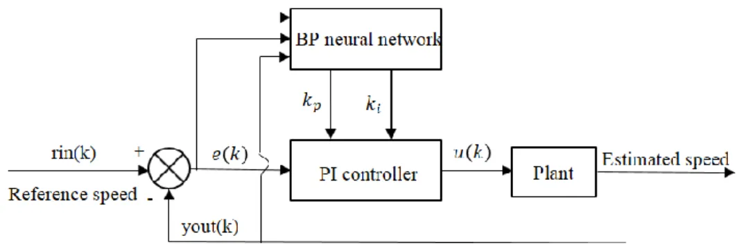
Fig. 11. The structure of NN-PI speed controller based on BP algorithm 21

Fig. 12. The BP neural network for proposed speed controller 21

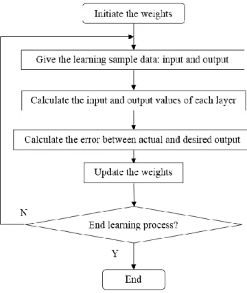
Fig. 13. The process of BP neural network 23

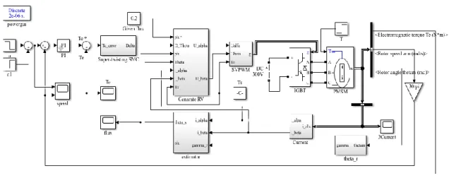
Fig. 14. Simulation block of STSM-DTC for IPMSM system 24

Fig. 15. Responses of torque(a) and flux (b)in steady state depending on variations ofk_P 26

Fig. 16. Responses of torque (a)and flux (b)in steady state depending on variations ofa 27

(11)

Fig. 17. Results of torque performances (a) and partial details of ZOOM-T2(b) 28

Fig. 18. Results of flux performances (a) and partial details of ZOOM-F1(b) 29

Fig. 19. Results of rotor speed performances 30

Fig. 20. Stator phase currenti_sa(A) of three control schemes 30

Fig. 21. FFT analysis and spectrum of THD for stator phase currenti_sa 31

Fig. 22. Simulation block of proposed control scheme for IPMSM 32

Fig. 23. Speed performances of PI and NN-PI controllers 33

Fig. 24. The auto-tuned parametersk_pandk_iof NN-PI speed controller 33

Fig. 25. The detailed figure of start-up speed responses in ZOOM-S1 34

Fig. 26. The detailed figure of steady-state speed responses in ZOOM-S2 35

Fig. 27. The detailed figure of speed tracking in ZOOM-S3 36

Fig. 28. Speed performance in case of load torque variation in ZOOM-S4 37

Fig. 29. Speed performance in case of load inertia variation 38

(12)

LIST OF TABLES

Table 1. The optimum voltage vector look-up table [19] 11

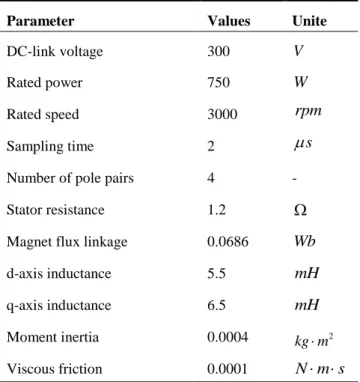
Table 2. System parameters 25

Table 3. The responses of torque and flux according to the variations ofk_P 26

Table 4. The responses of torque and flux according to the variations ofa 27

Table 5. The statistics of torque response in ZOOM-T1and ZOOM-T2 29

Table 6. The statistics of flux response in ZOOM-F1 30

Table 7. The statistics of start-up speed responses in ZOOM-S1 34

Table 8. The statistics of steady-state speed responses in ZOOM-S2 35

Table 9. The statistics of speed tracking in ZOOM-S3 35

Table 10. The statistics of robustness against load disturbance in ZOOM-S4 37

(13)

CHAPTER 1 INTRODUCTION

1.1 Background and Objectives

In recent years, the research and development on Electric Vehicles/ Hybrid Electric Vehicles (EVs/

HEVs) has become extensively popular due to the serious air pollution and the shortage of energy resources. For the electric propulsion systems in EVs/HEVs, the induction machine (IM), permanent magnet synchronous motor (PMSM), and switched reluctance motor (SRM)are usually considered [1].

However, owing to its outstanding advantages like high power density, high efficiency, simple structure and low maintenance cost, the PMSMs are extremely applied [2].

Inherent coupled flux and torque is the main disadvantage of PMSMs, which makes them hard to control. Many advanced control techniques have been presented to make PMSMs more comparable.

Filed-oriented control (FOC) [3] and direct torque control (DTC) [4] are the two main control techniques for PMSM drives. The FOC technique is widely used in PMSM drives. However, it performs not as well as predicted in practical engineering application due to the variations of motor parameters and inaccurate control mode [5]. In 1980s, DTC algorithm [6] was firstly introduced from ABB for induction motor drives. Decades past, it was already developed and used for variety of motor drives.

Compared with FOC, the conventional DTC is a significantly new concept with capability of controlling the electromagnetic torque and stator flux linkage directly. It has many characteristics of less dependence on machine parameters, fast dynamic response and less complexity without coordinate transformation or current regulation, and robustness against motor parameters’ variation and external disturbances [7]. Furthermore, it doesn’t need extra sensors to implement DTC. Hence, the DTC surpasses FOC in the application of EVs. However, as reported in literatures [2], [4], [7-12], this technique still possesses several major disadvantages, namely relatively large torque and flux ripples, variable switching frequency and high sampling requirement for digital implementation. Moreover,

(14)

the dynamic and stability of the system like improper speed response with high overshoot at the motor start stage, big speed ripples when system variations occur [11].

To solve the aforementioned-problems of conventional DTC, varieties of modified DTC schemes have been presented from various perspectives. One category is to add more available voltage vectors by using new hardware topologies. In [8], a multilevel convertor is employed to generate more voltage vectors for reducing torque ripples. However, it needs more power switches thus increasing the system cost and complexity. The category of nonlinear control technique was also presented. In [9-10], feedback linearization control (FLC) is used to convert the coupled nonlinear PMSM control system to an equivalent linear one. The FLC based DTC scheme in [10] achieves fast torque response and small torque and flux ripples. In these nonlinear FLC strategies, many motor parameters are used to get state variables. Hence, the robustness of the system will be deteriorated when parameters vary. Another category to enhance DTC scheme is the employment of space vector modulation (SVM) [2], [11], [13].

SVM based DTC can obtain voltage vectors with adjustable amplitude and phase, thus controlling the electromagnetic torque and stator flux more accurately. By incorporation with SVM, the DTC can be improved with torque and flux ripples reduction and fixed switching frequency. The fundamental issue of SVM based DTC is to get the reference voltage vectors. Some methods to obtain reference voltage vectors have been proposed in the literatures [2], [12-13].

All the strategies mentioned above are presented to improve the torque control of DTC controlled motors, but neglecting speed control which also plays an important role in electric machines. Generally, PI controller is widely applied in the outer speed regulator loop due to its relatively simple implementation and effectiveness [14]. However, the PI control approach cannot perform sufficiently well in nonlinear PMSM drives system with various uncertainties. Moreover, it’s time consuming and hard to tune the PI controller parameters which depends on the system [15]. Recently, some new methods have been proposed to replace PI speed controller. In [2], [9], sliding mode control (SMC) are applied in speed controller owing to its great merits such as robustness to external load disturbance and fast dynamic response. However, its system dynamics are still affected by parameter variations and chattering problems [18]. Meanwhile, adaptive speed control schemes are also proposed to control the

(15)

speed of PMSM [17-18]. With capability of automatic adjustment, adaptive control is the trend of digital control, but it’s hard to master the adaptive control law [15]. Next, the artificial neural network (ANN) is also an interesting scheme in the speed control of PMSM, due to its ability of approximate the linear or nonlinear mapping through learning. In [16], neural speed controller is designed and adopted to improve the control performances of vector control based PMSM. Nevertheless, only load torque variations and speed step change are considered.

In this thesis, a novel SVM based modified DTC algorithm by using predictive controller with super twisting sliding mode control (STSM) is adopted for electromagnetic torque and stator flux ripples reduction and fixed switching frequency, named as STSM-DTC method. Moreover, a novel adaptive speed controller based on neural network PI (NN-PI) is designed instead of a classical PI controller.

Consequently, simulation results demonstrate that proposed NN-PI speed controller combining STSM- DTC strategy can obtain high performance with fast dynamic response, small torque and flux ripples, small speed overshoot and speed drop against load torque and load inertia disturbance.

(16)

1.2 The mathematical modeling of IPMSM

This sub-chapter describes the basic mathematical modeling of PMSM in different reference coordinate.

(1) Modeling indqrotating frame

It’s convenient to design the control scheme when presenting IPMSM model indqrotating frame where d-axis coordinates with rotor at same speed. The equations of IPMSM in the rotating frame are shown as followings:

Stator voltage indqaxis:

d d n r q

q q d

d

q n r

Ri d p

dt

Ri d p

d u

u t

  

   



   



(1-1)

Stator flux indqaxis:

d q

d d f

q q

L i L i



 

 

 (1-2) Electromagnetic torque:

 

2

e 3 n d d d q f

T  p i ^i L L  ^ (1-3) Where

id,i_qstator current indandqaxis, Ld,L_qinductances ofdandqaxis,

 r rotor mechanical speed, pnnumber of pole pairs,

f permanent magnet flux.

(2) Modeling in  stationary frame

It’s complex to perform the mathematical modeling of IPMSM in stationary frame. Here give some equations as:

(17)

 



^u^u ^Ri^Ri



^dt^dt

  

  



  

  





 (1-4)

2 2

s  

    (1-5)

 

2

e 3 n

T  p _{ }i _{ }i (1-6) Where

u_,u_stator voltage of andaxis, i_,i_ stator current ofandaxis,

,_ stator flux ofandaxis, Rstator resistance,

 s amplitude of stator flux.

The dynamic equation is given as:

r



e L r



J d T T B

dt     (1-7) Where

Jcombined inertia of rotor and load

Bcombined viscous friction of rotor and load TLshaft mechanical (load) torque

(18)

1.3 Outline of the Thesis

The contents of the thesis are organized as follows:

In Chapter 2, the basic principle of the conventional DTC algorithm for IPMSM is introduced. Next, predictive calculator of voltage vector reference is presented and SVM technique is introduced briefly.

Finally, the super twisting sliding mode control is introduced and STSM based DTC technique (STSM- DTC) is designed.

In Chapter 3, the currently popular artificial neural network control is presented briefly at first. Then, the proposed neural network based PI speed controller (NN-PI) for IPMSM is designed and presented in detail.

In Chapter 4, simulation works are designed and introduced in various scenarios. In this part, the comparisons between proposed control strategies and other methods are introduced to demonstrate the effectiveness and the improvement of proposed algorithm.

In Chapter 5, conclusions and future works are presented.

(19)

CHAPTER 2 DTC FOR PMSM

2.1 Review of Classical DTC

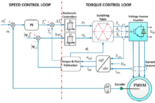
DTC is a significant new concept developed by ABB company. In this scheme, the motor parameters, namely electromagnetic torque and flux are being controlled directly. It doesn’t need a modulator, as used in PWM drives, to control the frequency and voltage. The schematic of conventional DTC for PMSM is shown in Fig. 1. It includes two parts, namely speed control in the outer loop and torque control in the inner loop. It usually consists of a proportional-integral (PI) speed controller, two hysteresis controllers for electromagnetic torque and stator flux regulation, heuristic switching table for generating a variable switching frequency and electromagnetic torque and stator flux estimator. The principle of DTC for voltage source inverter (VSI)-fed PMSM is presented in the followings of this section.

Fig. 1. Block diagram of the conventional DTC for PMSM.

Firstly, the principles of torque control will be presented. Fig. 2. shows some vector in different reference frames. The stator flux for a PMSM indqrotating coordinate are given as:

(20)

cos sin

d q

s s

 



 

 

 

 (2-1) Where is torque angle between stator flux and permanent magnet flux.

According to the formula (1-2) and (2-1), the stator current of referencing todqaxis can be expressed as:

cos sin

d f s f

d

q s

q q

d

q

d

i i

L L

    

  

  

 



  



(2-2)

Based on the equations (1-3) and (2-2), the torque can be described as the following equation [2]:

3( ) 2

3 sin sin 2

2 4

d q

n

e s f s

d d q

L L T p

L    L L  

  (2-3)

Fig. 2. Relationship between different quantities in different reference frames.

In a control period, rotor flux changes slowly due to its dependence on a relatively large rotor time constant; therefore, it can be assumed to be constant in short time. In DTC control scheme, the stator flux amplitude is also a constant value. From equation (2-3), it can be concluded torque can be changed if the instantaneous positions of the stator flux vector are changed quickly so that the torque angle is altered as quickly as possible [19]. This is the basis of DTC method. The stator flux vector instantaneous change can be achieved by switching on the appropriate stator voltage space vector of the VSI. The stator flux vector in stationaryA B C  coordinate can be expressed as following:

 

s us R i dts s

 



 (2-4)

(21)

Whereu_s and i_s are stator voltage vector and current vector in stationary A B C  coordinate. If neglecting the stator resistance voltage dropping, in a short period of time the relationship between incremental_sandu_sis proportional, given as:

s us t



   (2-5) From (2-5), we can infer that changing rate of_sis nearly same to that ofu_s. If define_s _s e^j^^s , where_sis the position angle of stator flux vector referenced toAaxis, as shown in Fig. 2. Then the stator voltage vector can be described as:

1 2 ^s

s j

s s s s s

u u u d e j

dt

 

 

    (2-6)

Where _s ^d ^s dt

   is rotating speed synchronous to_s. As shown in (2-6) and Fig. 2., u_shas two parts, namelyu_s₁andu_s₂. u_s₁coincides with_s; therefore, it can only change the amplitude of_s. How the stator flux is kept within a hysteresis band _s by selecting the voltage vectors is shown in Fig. 3. u_s₂ is perpendicular to_s; therefore, it can only control the rotating speed_sof_s, then finally control the electromagnetic torque. This the reason that DTC has the merit of fast dynamic control.

Fig. 3. Space voltage vectors and application to control stator flux space vector and torque.

As shown in Fig. 3., there are six sections with 60 degrees from₁to₆and only six active voltage vectors (two zero voltage vectors) V_i (i1, 2,3....8), named the space vectors of inverter output phase voltages. It also illustrates that how the VSI output voltage vectors effect on the stator flux and torque,

(22)

where the stator flux vector_sis located at sector₁and rotate anticlockwise. The currently applied voltage vector isu_s. The selection process of voltage vectors is determined by inverter operation. If voltage vectorV₂(110) is selected, the torque and stator flux magnitude will be increased simultaneously.

If voltage vector V₅(001) is selected, the torque and stator flux magnitude will be decreased simultaneously. If applyingV₃(010), the torque will be increased but stator flux magnitude is decreased.

Similarly, if applyingV₆(101), the torque will be reduced and stator flux magnitude is increased. This kind analysis can be extended similarly to the other sectors accordingly [2]. According to above analysis, the stator flux vector and torque can be controlled by using appropriate stator voltage space vectors, obtained from the VSI controlled by switching table, as shown in Fig. 3. Obviously, switchover of voltage vectors is operated step by step, and the stator flux vector is nearly the integration of voltage vector (2-4), thus the angle between stator flux and voltage vector varies step by step. However, the position of stator flux vector is continuously varying during the motor rotor rotates in practice. Hence, conventional DTC has the relatively large ripples in torque and flux.

The status of switchesS_a,S_bandS_cof switching table decide the inverter output voltage space vectors.

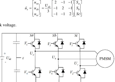
Fig. 4. shows the two level, three-phase VSI-fed PMSM system. The relationship between three-phase stator voltage vectoru_sand switching statesS_a,S_bandS_ccan be described as equation (2-7). The optimum switching table of eight-voltage vector for controlling_sandT_eshown in Table 1.

2 1 1

1 2 1

3 1 1 2

sa a

dc

s sb b

sc

u S

u u U S

u Sc

 

     

     

      

        

 

(2-7)

WhereU_dcis dc-link voltage.

Fig. 4. Typical topology of three-phase VSI for PMSM.

(23)

The_s,T_eand_sare the inputs of switching table._sandT_eare generated by torque and flux hysteresis controllers respectively, which are described as following:

0 4444 4444

1 _s _s _s

s s s

s

if if

  





   



 



 (2-8)

555555 555555 1

1

555555 44 4

0 4

e

e e e

e e

e e e

ifT T T

ifT T

T





   

 

   



 

(2-9)

Where _s^ and T_e^ are reference stator flux magnitude and reference electromagnetic torque respectively._sandT_eare hysteresis band of stator flux magnitude and reference electromagnetic torque respectively.

Table 1. The optimum voltage vector look-up table [19]

s T_e ₁ ₂ ₃ ₄ ₅ ₆

1

1 V2 V₃ V₄ V₅ V₆ V₁

0 ^V⁷ V8 V₇ V₈ V₇ V₈

-1 ^V⁶ V1 V₂ V₃ V₄ V₅

0

1 ^V³ V4 V₅ V₆ V₁ V₂

0 ^V⁸ V7 V₈ V₇ V₈ V₇

-1 ^V⁵ V6 V₁ V₂ V₃ V₄

In the speed control loop, the reference torque is generated by the PI speed controller that regulate the speed error between reference speed and estimated speed.

(24)

2.2 Proposed STSM-DTC Technique Design

(1) Generation of Reference Voltage Vector

As introduced in section 2.1, the basic principle of DTC is to select the optimal voltage vectors, which makes the stator flux linkage space vector rotates to required position while keeping magnitude within limited and generate desired torque. However, the conventional DTC suffers the limited number of voltage vectors with changeless amplitude and fixed direction [2]. The SVM algorithm will be adopted to control the VSI generate more reference voltage vectors. It can regulate the stator flux and torque more precisely with fixed switching frequency when incorporating with SVM technique [10].

In stationary   reference frame, reference flux vector calculator (RFVC) [12] is employed to produce reference stator flux vector_ref, then used for generating desired voltage vectoru_ref , as shown in Fig. 5. At sample timek, estimated stator flux amplitude_s( )k and its position angle_s( )k can be calculated from flux estimator. Then at next timek1,these values become_s(k1)and_s(k1). The incremental angle_sbetween_s( )k and_s(k1)is generated by STSM torque controller. If define

( 1)

s k

  as same to given stator flux amplitude_s^, and_s( )k _s. Then_s(k1)and_s( )k can be described as followings:

Fig. 5. Signal flow chart of generating reference flux vector [27].

(25)

cos( ) ( 1)

( 1)

( 1) sin( )

s s

s

s s

k k

k





  

    



   

    

        

(2-10)

( ) cos( )

( ) ( ) sin( )

s s

s

s s

k k

k





  

   

 

   

    (2-11) Through the discretization of equation (2-4), the stator voltage vector can be transformed as following:

( 1) ( )

( 1) ^s ^s

s s

s

k k

u k i R

T

  

   (2-12) WhereT_sis the sampling interval.u k_s( 1)is the desired voltage vector, namely reference stator voltage vectors. From equations (2-10), (2-11) and (2-12), we can get the reference voltage vector in  stationary reference frame as:

cos( ) cos( )

sin( ) s

( )

( ( )

) in

ref

s

re

s s s s

s

s s s

f

u Ri k

T

u Ri k

T

 

 

    



 

  



 

   

 



(2-13)

By specifying a reference voltage vector, the SVM (space vector modulation) technique is used to determine action time and produce switching control signals to be applied to the inverter [10]. Thus, a voltage vector will be reconstructed by switching on two adjacent vectors for proper time. One example that the reference voltage vector locates at sector I is shown in Fig. 6., where the vectoru k_s( 1)can be obtained by the different switching on/off sequence of fundamental voltage vectorsV V₁/ ₂/V₀with time durationT T₁/ ₂/T₀. This is the basis of SVM, called as average equivalence principle, as described in equation (2-14). This proposed DTC with SVM technique still retains all the advantages of conventional DTC by replacing two hysteresis controllers with a STSM torque controller and predictive controller, the switching table with a SVM.

1 1 2 2 0 0 ( 1 2 0 )

s s s

T u TVT V T V T T T T (2-14)

Fig. 6. Reference voltage vector as a combination of adjacent vectors at sector I.

(26)

(2) Design of Super-twisting SMC based Torque Controller

As known from the equation (2-3), the relation between the error of torque and the incremental of torque angle is nonlinear. In [12], the classical PI controller is applied to produce the torque angle increment required to minimize the error between reference torque and estimated torque. However, as mentioned before, the PI controller performs in nonlinear systems is not as good as that in linear systems.

In this paper, a novel super-twisting sliding mode (STSM) controller is designed and used to regulate the angle increment of which is linear to . The super twisting is a modified second order sliding mode algorithm that can reduce the chattering effect while retaining the other properties of conventional SMC. Moreover, it does not need the information of any derivative of the sliding variable [9]. The general STSM control law contains two parts, one is a discontinuous function of the sliding variable, and the other is a continuous function of its derivative with respect to time, given as [25]:

1 1

sgn( ) sgn( )

r

ST P

I

u k y y u

du k y

dt

  

 





(2-15)

Where the k_Pand k_Iare positive gains used to adjust the STSM controller. The degree of nonlinearity of system can be adjusted by the positive coefficient (0r  r 0.5). The sufficient condition for a short time convergence to the sliding surface and stability are given by Levant in [26] as:

m

2 m

4 ( )

( )

M I

M M I M

P

m I M

k A B

A B k A

k B B k A









 

 



(2-16)

WhereA_M Aand B_M  B B_m,whereAandBare defined by the second derivative ofy:

2

2 ( , ) ( , )

d y du

A x t B x t

dt   dt (2-17) The first derivative of electromagnetic torque in equation (2-3) can be described as:

3 2 cos 2 ( ) cos(2 )

4

n s

e

f q s q d

d q

dT p

L L L

dt L L

        

     (2-18)

It can be inferred that its second derivative contains the torque angle second derivative, that is torque angle incremental first derivative. Also the quantitiesAandBin (2-17) are both bounded, since the stator flux magnitude_s and inductionsL_d ,L_qare constants. As indicated in [12] that

(27)

s n r

 T p 

    , where electrical angular speed_ris also limited. Therefore, STSM controller for angle incrementalcan be designed as:

1

2 1

1

tanh( ) tanh( )

P Te Te

I Te

k s as u

du k as

dt



  

 





(2-19)

Where hyperbolic tangent function tanh( ) ( 0)

ax ax

e e

ax a

e e



  

 is adopted to replace the switching function sgn( )x which has strong discontinuity causing chattering. The applied tanh(ax)is continuous function with smoother variation of curve slope rate, which can eliminate the chattering. The coefficient

adetermines slope rate. The sliding variable is the torque errors_TeT_e^*T_ebetween reference torque and actual torque. The gainsk_Pandk_Ishould fulfill the stability condition in equation (2-16). The diagram of proposed STSM torque controller is shown in Fig. 7. This modified DTC scheme is named as STSM-DTC in this paper.

Fig. 7. The schematic of proposed STSM torque controller.

(28)

CHAPTER 3

SPEED CONTROLLER BASED ON ANN

3.1 ANN Control Technique

Natural neurons, the simple computational units of brain, which are interconnected in complex manner. Many interconnected neurons constitute neural network that can solve complex problems, replicate responses and generalize signal. Inspired by this, artificial neuron and ANN are created.

Fig. 8. shows the natural neural and artificial neuron. The artificial neuron basically consists of three parts. At the entrance, inputs are multiplied by individual weights that means strength of the respective signals. and then. In the middle, all previously weighted inputs and bias will be summed. At the exit of artificial neuron, the summed values will be computed by a mathematical function, namely activation function of the neuron [20].

Fig. 8. Biological neuron (left) and artificial neuron (right).

ANN can be built to solve complex problems when combining two or more artificial neurons.

According to the way of artificial neurons’ interconnection, ANNs are classified into two basic types, Feed-forward Neural Network (FNN) and Recurrent Neural Network (RNN). The simple examples of three-layered FNN and RNN are shown in Fig. 9. Multi-Layer Perceptron Neural Network (MLPNN)is one typical FNN, which can be used to represent any nonlinear mapping to an arbitrary degree of

(29)

accuracy. In this paper, the MLPNN is adopted in motor speed control.

Fig. 9. The topology schematic of three-layered FNN (left) and RNN (right).

As known that biological neural networks can tell how to respond to the given inputs from the environment properly after learning. Therefore, to get the expected outputs from ANNs, we need to teach the ANNs how to learn from processing experience. There are three major learning paradigms, namely supervised learning, unsupervised learning and reinforcement learning. All these learning method target to set the values of weight and biases on basis of learning data to minimize the chosen cost function [21]. Supervised learning is a widely used machine learning technique. Its task is to set parameters of an artificial neural network based on the training data which consists of inputs and desired outputs.

The Back-Propagation (BP) algorithm is the most common learning algorithm of supervised learning technique, typically using gradient descent method. The idea of BP algorithm is to reduce the error between actual outputs and expected results, until the ANN learns the training data [20]. The structure of a three-layer BP neural network is shown in Fig. 10.

Notation states:

• n_l: number of neurons in l^thlayer;

• ^f

 

^• : activation of neuron;

• W^{( )}^l  ^{n n}^l^^l^¹: weights vector from (l1)^thlayer to l^thlayer;

• w ^{( )}^l : the element of weights vectorW^{( )}^l , representing the weight between j^thneuron in

(30)

(l1)^thlayer andi^thneuron inl^thlayer;

• ^b^{ }^l ^



^b¹^{ }^l ^,^b²^{ }^l ^, ^,^bⁿ_{ }^l^{ }^l



^^ ⁿ^{ }^l : the bias between(l1)^thlayer andl^thlayer;

• ^{ } ^{ } ^{ }

 



¹ ^, ² ^, ^, ^l 



ⁿ^{ }^l

l l l l

z z zn

 

z : states of neurons inl^thlayer;

• ^a^{ }^l ^



â¹^{ }^l ^,â²^{ }^l ^, ^,âⁿ^l^{ }^l



^^ ⁿ^l: outputs of neurons inl^thlayer.

Fig.10. The structure of BP neural network.

If the BP neural network is a three-layered model withjinputs,ihidden nodes andkoutputs. Then the work process of BP algorithm is given as following [22]:

Step 1: Initialize weight to small random values.

Step 2: While stopping condition is false, do steps 3-10.

Step 3: For each training pair do steps 4-9.

Feedforward pass

Step 4: the state vector and activation vector in^l^th



²^{ }^l ^L



layer is expressed as:

       

 

1

l l l l

l l

f

  



z W a b

a z (3-1) For a L^thlayer perceptron, the final output of network is a^{ }^L . The feedforward process of

information is described as:

 ¹  ² ^L¹  ^L  ^L

     

x a z a z a y (3-2)

(31)

Backward pass

Step 5: Set the training data as

 x 1,y 1 ,x 2 ,y 2 , x i ,y i , x N ,y N  

^with^Ndata sets, and

 ⁱ ^



^y¹ ⁱ ^, ^,^y^nL ⁱ



^

y . For one training data



^x^{ }ⁱ ^,^y^{ }ⁱ



, the cost function is as following:

     



   



²

1

1 1

2 2

i i nL i i

k k

i

k

E y o



 ^y ^o 



 (3-3)

Wherey^{ }ⁱ is the expected output vector, o^{ }ⁱ is the actual output vector according to the input ofx^{ }ⁱ . If expand the equation (3-3) to hidden layers and finally input layer, we will find that the cost function is only related to weights vectorW^{ }^l and bias vectorb^{ }^l , which means that adjusting the values of weights and bias can reduce or enlarge the error. Obviously, the totally averaged cost of all training data is:

 

1

1 ^N

total i

i

E E

N _





(3-4)

Step 6: Update the weights and bias ofl^thlayer from time t to t1 by using gradient descent method.

The iteration updating equations of parameters are given as:

  

     

  

1 1

1

55555

l l l

t t t

N i t

l

t l

i t

E N



 



  

  





W W W

W

(3-5)

  

     

  

1 1

1

5555

l l l

t t t

N i t

l

t l

i t

E N



 



  

  





b b b

b

(3-6)

Where  is learning rate.

(32)

3.2 Proposed NN-PI Speed controller

Inspired by the amazing function of neurons, the artificial neural network (ANN) has been developed very fast to solve big scale and complex problems recently. Numerous works [16], [23-24] have demonstrated that ANN is suitable for dynamic and nonlinear control systems due to the capability of processing, analyzing and learning. The speed controller of DTC structure is a nonlinear system, which has disturbances of load inertia and motor parameters variation against temperature [17]. This makes it difficult for PI speed controller to perform sufficiently well for this DTC control system. This paper proposes an adaptive speed controller based on back propagation (BP) neural network, which is verified by simulation with high performances.

The PI control theory has been one of the most widely used methods in industrial application. In a continuous-signal system, the PI equation is expressed in (3-7). When the sampling period is very small, a discrete-time PI controller can be obtained as (3-8) by replacing integrate with summation and replacing derivative with difference quotient of (3-7).

0

( ) ( ( ) 1 ( ) )

t p

i

u t k e t e d T  

   (3-7)

0

( ) ( ( ) ( ))

s k p

i j

u k k e k T e j T 

   (3-8) Where ( )u t and ( )u k are controller outputs in the inner training loop at continuous-timetand discrete- timek, respectively; ( )e t and ( )e k represent tracking errors at continuous-timetand discrete-timek, respectively;k_pis proportional gain;T_iis integral time constant;T_sis the sampling period. However, the calculating of integral part in equation (3-8) needs to accumulate all errors in the past, which takes huge storage and time. For convenience program coding work, equation (3-8) can be described as incremental form as following [24]:

   

1111

( ) ( 1) ( )

( 1) _p 1 _i

u k u k u k

u k k e k e k k e k

   

      (3-9) Wherek_iis the integral gain.k_pandk_iare auto-tuning parameters depending on the system states. The equation (3-9) can be described as:

( ) [ ( 1), _p, , ( ), (_i 1)]

u k  f u k k k e k e k (3-10)

(33)

Where ( )f • is a kind of nonlinear function related to (u k1), ( ),y k k k_p, _i. BP neural network can find the best control rule of ( )f • through training and learning.

The NN-PI speed controller using error backpropagation (BP) algorithm consists of two parts. One is classical PI controller which can regulate motor speed in the closed loop. The other is BP neural network which can tune the parameters ofk_pandk_ionline to achieve the optimal performance [28]. The schematic structure of NN-PI speed controller is shown as in Fig. 11.

Fig. 11. The structure of NN-PI speed controller based on BP algorithm.

This NN-PI speed controller adopts a three-layers BP neural network with 3 input-neurons in input layer, 5 hidden-neurons in hidden layer and 2 output-neurons in output layer, as shown in Fig. 12. The inputs are set as reference speed, actual speed and error between them. Thek_pandk_iare non-negative outputs of network. Sigmoid function is selected as the activation function of output layer.

(34)

Based on the section 3.1 and Fig. 12., the equations for proposed NN-PI speed controller are given as:

(1)_j

( )

_j

( )

555555585

( 1, 2,3)

a k x k j (3-11)

(2

3

(2) (2) (1)

1 (2) )

( ) ( )

( ) ( ( ))555555( 1, 2,3, 4,5)

i ij j

j i i

z k w a k

k f k i

a z



 



(3-12)

2

(3) (3) (2)

1

(3) (3)

( ) ( )

( ) ( ( ))555 585 5( 1,2)

k ki i

i

k k

z k w a k

a k g z k k



 



(3-13)

   

( ) tanh( ) ( ) 1 1 tanh

2

x x

x

x x

e e

f x x

e e

g x x e

e e



  



  



(3-14)

Wherez_n^{( )}^l anda^{( )}_n^l present the summed input values and output ofn^thneuron inl^thlayer, respectively.

( )l

wnm denotes the connection weight betweenm^thneuron in(l1)^thlayer andn^thneuron inl^thlayer. ( )f x and ( )g x are activation function for hidden and output layer, respectively. The backpropagation pass is described as followings.

(3) (3)

(3)

( ) ( ) ( 1)

ki ki

ki

w k E k w k

^w 

     

 (3-15) Wherew_ki⁽³⁾( )k is weight incremental quantity of output layer with an additional momentum for fast convergence.is momentum coefficient. ( )E k is cost function. According to the chain rule of derivative, the partial derivative of error to weight can be expressed as:

(3) (3)

(3) (3) (3) (3)

( ) ( )

( ) ( ) ( ) ( )

. . . .

( ) ( ) ( ) ( )

k k

ki k k ki

a k z k

E k E k y k u k

w y k u k a k z k w

 

   

      (3-16)

Wherein ( )y k stands for the actual outputs; ( ) ( ) y k u k



 is unknown as the model is unknown. But the variation amounts of ( )y k and ( )u k can be obtained. Therefore, the sgn( )• , that determines the direction of weights varying, can be employed to get the approximate value. The caused uncertainty can be compensated by adjusting learning rate. According toa₁⁽³⁾k_p, a₂⁽³⁾ k_i and equation (3-9), we get:

(35)