Supply Chain Inventory Model for Items with Stock
Dependent Demand Rate and Exponential Deterioration under Order-Size-Dependent Delay in Payments
Seong Whan Shinn*
*Department of Industrial Engineering, Halla University
주문량 종속 신용거래 하에서 재고 종속형 제품수요를 갖는 퇴화성제품의 공급체인 재고모형
신 성 환*
*한라대학교 산업경영공학과
Abstract
본 연구는 공급자(supplier), 중간공급자(distributor) 그리고 고객(customer)으로 구성된 2 단계 공급사슬에서 퇴화성 제품(deteriorating products)에 대한 중간공급자의 재고모형을 분석하였다. 문제 분석을 위해 공급자는 중 간공급자의 수요 증대를 목적으로 중간공급자의 주문 크기에 따라 차별적으로 외상 기간을 허용하고, 최종 고객의 수요는 중간공급자의 재고 수준에 따라 선형적(linearly)으로 증가한다는 가정 하에 모형을 분석하였다. 중간공급자 의 이익을 최대화하는 경제적 주문량 결정 방법을 제시하였고, 예제를 통하여 그 해법의 타당성을 보였으며, 민감 도 분석을 통하여 퇴화율이 재고정책에 미치는 영향을 분석하였다.
Keywords: Inventory, EOQ, Order-size-dependent delay in payments, Stock dependent demand rate, Exponential deterioration
1. Introduction
In this paper, we extend the model presented by Shinn [11] to the case of deteriorating products. We consider a two-stage supply chain which consists of the supplier, the distributor(wholesaler/retailer) and his customer. The purpose of this paper is to evaluate the distributor's inventory system in which his customer’s demand rate of the product is a function of the distributor’s on–hand inventory level (quantity on–hand) and the supplier offers a credit period to the distributor assuming that the supplier’s credit terms are already known and the length of delay in payments is a function of the amount purchased. It is also assumed that inventory
is depleted not only by customer’s demand, but also by deterioration.
According to Shinn [11], it is very common to see that the distributors are allowed some grace period before they settle the account with their supplier. In this regard, there were a number of research papers in the literature. Goyal [4] and Teng et al. [12] analyzed the mathematical model for obtaining the EOQ (economic order quantity) model when the supplier permits a fixed delay in payments with single-credit period. Chang et al. [2], and Kreng and Tan [5] evaluated the inventory model under two levels of trade credit policy depending on the order quantity (multiple - credit periods).
†Corresponding Author : Seong Whan Shinn, E-mail: [email protected]
Received July 15, 2015; Revision Received September 08, 2015; Accepted September 11, 2015.
Ouyang et al. [9] analyzed the joint pricing and
ordering problems in a supply chain under multiple-credit periods assuming that the demand rate is a function of the retailer's selling price.
Recently, Shinn [11] has evaluated the distributor's inventory model under multiple-credit periods in payments assuming that the customer's demand rate is dependent on the distributor's inventory level.
Some research papers evaluated an inventory system where the demand rate has been assumed to be dependent on the on-hand inventory. Among the important research papers published so far with stock dependent demand rate, mention should be made of works by Baker and Urban[1], Mandal and Phaujdar [7, 8], Padmanabhan and Vrat [10]
and Shinn[11]. Baker and Urban [1] evaluated an inventory system assuming the demand rate to be a polynomial functional form of the on-hand inventory level at that time. Mandal and Phaujdar [7] also discussed an inventory system assuming the demand rate to be a linear function of the on-hand inventory level at that time. Shinn [11]
also, has evaluated the distributor's inventory model for a product assuming the demand rate to be a linear function of the on-hand inventory level under multiple-credit periods in payments.
All of the research mentioned above implicitly assumes that inventory is depleted by customer’s demand alone. This assumption is quite valid for non-perishable or non-deteriorating inventory items. However, there are numerous types of inventory whose utility does not remain constant over time. In this case, inventory is depleted not only by customer’s demand but also by deterioration. In this regard, assuming the exponential deterioration of the inventory in the face of constant demand, Ghare and Schrader [3]
derived a revised form of the economic order quantity. Also, Mandal and Phaujdar [8], and Padmanabhan and Vrat [10] analyzed an inventory model for deteriorating products where the customer’s demand rate has been assumed to be dependent on the on-hand inventory. Recently Mahata and Goswami [6], and Tsao and Sheen [13] also extended the inventory model to the
case of deteriorating products under the condition of permissible delay in payments.
In view of this, this paper deals with the problem of determining the distributor's EOQ for an inventory-level-dependent demand rate items assuming that the supplier’s credit terms are already known and the length of delay in payments is a function of the amount purchased(multi-credit periods). For the analysis, we also assume that inventory is depleted not only by customer’s demand, but also by deterioration. In the next section, we formulate a relevant mathematical model. The properties of an optimal solution are discussed and a solution algorithm is given in Section 3. A numerical example and a sensitivity analysis are provided in Section 4, which is followed by concluding remarks in Section 5.
2. Model Development
This study examines the inventory model under multi-credit periods assuming that the demand rate is a function of the on-hand inventory level. The objective of this paper is to find the distributor’s EOQ which maximizes his annual net profit.
2.1. Assumptions and notations
The assumptions and notations of this paper are essentially the same as the model stated by Shinn [11] except for the condition of deterioration. The mathematical model is developed on the basis of the following assumptions :
(1) Replenishments are instantaneous with a known and constant lead time.
(2) No shortages are allowed.
(3) The inventory system involves only one item.
(4) The demand rate is linearly dependent on the level of inventory.
(5) The supplier allows a delay in payments for the products supplied where the length of delay is a function of the distributor’s total amount of purchase.
(6) The purchasing cost of the products sold
during the credit period is deposited in an interest bearing account with rate I. At the end of the period, the credit is settled and the retailer starts paying the capital opportunity cost for the products in stock with rate R(≥) (7) Inventory is depleted not only by demand but also by deterioration. Deterioration follows an exponential distribution with parameter .
The following parameter notations are used : C : unit purchase cost.
P : unit selling price.
S : ordering cost.
H : inventory carrying cost, excluding the capital opportunity cost.
R : capital opportunity cost (as a percentage).
I : earned interest rate (as a percentage).
Q : order size.
T : replenishment cycle time.
: credit period set by the supplier for the amount purchased CQ, ≤ , where
, ⋯ and ⋯ ,
, ∞.
: a positive number representing the inventory deteriorating rate
q(t): inventory level at time t.
D : annual demand rate, as a linear function of the on-hand inventory, where and are non-negative constants.
2.2. Proposed model development
For the model development, the analysis will concentrate on the situation in which the customer's demand rate is represented by a linear function of the on-hand inventory. That is, the demand rate at time t, will take the form:
, ≥ . (1) For the case of exponential deterioration as stated by Ghare and Schrader [3], the rate at which inventory deteriorates will be propotional to on hand inventory, q(t). Thus, the depletion rate of inventory at any time t is
, (2) Equation (2) is a first order linear differential equation and its solution is equation (3).
. (3)
Equation (3) gives an inventory level after time t due to the combined effects of demand usage and exponential deterioration. Note that due to the inventory carrying costs, it is clearly optimal to let the inventory level reach zero before reordering, i.e., q(T) = 0. So, given that q(T) = 0,
. (4)
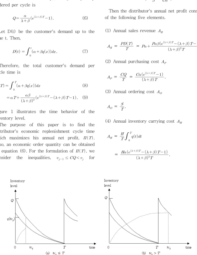
[Figure 1] Inventory level(q(t)) vs. Time(t).
And then,
, ≤ ≤. (5)
Also, from the fact that q(0) = Q, the quantity ordered per cycle is
. (6)
Let D(t) be the customer's demand up to the time t. Then,
. (7) Therefore, the total customer's demand per cycle time is
(8)
. (9)
Figure 1 illustrates the time behavior of the inventory level.
The purpose of this paper is to find the distributor's economic replenishment cycle time which maximizes his annual net profit, . Also, an economic order quantity can be obtained by equation (6). For the formulation of , we consider the inequalities, ≤ for
⋯ . Using equation (7), the inequalities can be reduced to
≤ , ⋯ where
. (10)
Then the distributor's annual net profit consists of the following five elements.
(1) Annual sales revenue
=
=
.
(2) Annual purchasing cost
=
=
.
(3) Annual ordering cost
=
.
(4) Annual inventory carrying cost
=
=
.
[Figure 2] Credit period() vs. Replenishment cycle time(T).
(5) Annual capital opportunity cost for
≤ :
(i) Case 1(≤): (see Figure 2. (a)) As products are sold, the sales revenue is used to earn interest with annual rate I during the credit period . And the average number of products in stock earning interest during time is
and the interest
earned per order becomes
. When the credit is settled, the products still in stock have to be financed with annual rate R. Since the average number of products during time becomes
and the interest payable per order can be expressed as
,
=
.
(ii) Case 2(): (see Figure 2. (b)) For the case of , all the sales revenue is used to earn interest with annual rate I during the credit period . The average number of products in stock earning interest during time is
. Therefore,
=
Then, the annual net profit can be expressed as
= .
Depending on the relative size of to T, has two different expressions as follows:
1. Case 1 (≤)
=
-
-
-
-
+
+
, ⋯ , (11)
2. Case 2 ()
=
-
-
-
+
-
-
+
, ⋯ . (12)
3. Determination of Optimal Policy
In this model, we want to find an optimal replenishment cycle time which maximizes
. Recognizing that the model has a very complicated structure, the model can be solved approximately by using a truncated Taylor series expansion for the exponential function, i.e.,
≈
, (13)
which is a valid approximation for smaller values of . Thus, using the Taylor series approximation the annual net profit function can be rewritten as:
= -
-
, ⋯ , (14)
= -
-
, ⋯ . (15) Note that for the case with , equation (14) and (15) are the same results as those by Shinn [11] for non-deteriorating product.
Now, we can consider the necessary and sufficient conditions for maximizing with respect to T.
The first order condition with respect to T is:
=
+
, (16)
=
+
. (17) Then, the second order condition with respect to T is:
=
, (18)
=
. (19)
For the normal condition(≥) stated by
Goyal[4],
for and
⋯ . Therefore, is a concave function of T and so, there exists a unique value
, which maximizes and they are:
=
where and
,(20)
=
where . (21)
Developing a solution algorithm, we investigate the characteristics of , and
⋯ . From equations (14) and (15), the annual net profit at has the following relation:
, ⋯ . (22) And we can make the following properties about and . These properties simplify our search process to find an optimal replenishment cycle time which maximizes the annual net profit function, .
Property 1. For and ⋯ ,
. (23)
Proof. From equations (20) and (21), we can show that
, and ⋯ , and so is an increasing function of . Therefore
holds since . Q.E.D.
Property 2. There exists at least one ∈ for and ⋯ .
Proof. From equation (23), if there were no
∈ for and ⋯ , either
≥ or for every i and j. Hence, either ≥ or holds, which contradicts the feasibility of T, i.e., ∞. Q.E.D.
Property 3. For any T, , for
and ⋯ .
Proof. From equations (14) and (15), we can show
that
, and ⋯ , and so the annual net profit function is an increasing function of . Therefore holds
since Q.E.D.
Now, we can know that the characteristics of the annual net profit are essentially the same as non-deteriorating case stated by Shinn [11]
except for the structure of equations, and
. Based on the above results, we can apply the same solution procedure to determine an optimal replenishment cycle time .
Solution algorithm
Step 1.Compute by equation (20) and find the largest index a such that ∈ for ⋯ .
Step 2.(for the indices ) In case
2.1 , then compute the annual net profit with equation (14) for . 2.2 ≤ , then compute the annual
net profit with equation (14) for . 2.3 ≤ , then there exists no candidate
value of the maximum annual net profit for ∈ .
Step 3. (for the index ) In case
3.1 , then compute the annual net profit with equation (14) for and go to Step 5.
3.2 ≤ , then compute the annual net profit with equation (14) for and go to Step 4.
3.3 ≤ , go to Step 4.
Step 4.(for the indices ) In case
4.1 and ≤, then compute the annual net profit with equation (14) for
and go to Step 5.
4.2 and max ≤ , then compute the annual net profit with equation (14) for and go to Step 5.
4.3 and max , then compute the annual net profit with equation (14) for max .
4.4 ≤ , then there exists no candidate
value of the maximum annual net profit for∈ .
Step 5.Compute by equation (21) and find the largest index b such that ∈ for ⋯ .
Step 6.If , then compute the annual net profit with equation (15) for and go to Step 7. Otherwise, go to Step 7.
Step 7.(for the indices )
If ≥ , then compute the annual net profit with equation (15) for . Otherwise, there exists no candidate value of the maximum annual net profit for
∈ .
Step 8.Select the replenishment cycle time() with the maximum annual net profit value evaluated in previous steps.
4. Numerical Example and Sensitivity Analysis
Comparing the model with the case of non-deterioration as stated by Shinn [11], the same example problem is solved except for the deteriorating rate .
(1) C = $20, P = $23, = $100, H = $5, R = 0.15( = 15%), I = 0.1( = 10%), ,
and .
(2) Supplier's credit schedule:
Total amount of purchase(order size) Credit period ≤ ≤
≤ ≤
≤ ≤
≤ ∞ ≤ ∞
In order to solve the problem, a computer program written in QBASIC was developed to find an optimal solution for the approximate model.
As a result, the solution procedure generates an optimal solution, for the approximate model and an optimal lot size, can be obtained by equation (6) as follows;
Replenishment cycle time () = 0.1527 year;
Economic order quantity ()=508 units;
Maximum annual net profit ()=$8441.46 .
An interesting question to ask is how much effect the size of the deteriorating rate () has on the distributor's decision. Also, we want to know the effect of on the distributor's decision. Since the structure of equations (14) and (15) does not permit sensitivity analysis, the same example problem is solved to answer the above question.
Five levels of are adopted, = 0.1, 0.2, 0.3, 0.4 and 0.5. For each level of , six levels of , ranging from 0.0 to 0.5 with an increment of 0.1, are tested. The results are shown in Table 1 and the following observations can be made, which are consistent with our expectations:
(i) With fixed, as increases, does not increase and decreases.
(ii) With fixed, as increases, does not decrease and increases.
(iii) With fixed, as increases, and increases.
Note that for the case with and , the algorithm generates the same results as those by Shinn [11].
<Table 1> Sensitivity analysis with various values of and
0 . 0 0 . 2 0 . 3 0 . 4 0 . 5
0.1527
492 9242.83
0.1527 496 9330.79
0.1527 500 9418.74
0.1527 504 9506.70
0.1527 508 9594.65
0.1527
496 8754.19
0.1527 500 8842.15
0.1527 504 8930.10
0.1527 508 9018.06
0.1527 512 9106.01
0.0766
248 8268.03
0.1527 502 8353.51
0.1527 508 8441.46
0.1527 512 8529.42
0.1527 516 8617.37
0.0703
228 8033.53
0.0712 232 8072.01
0.0722 236 8111.03
0.0733 241 8150.60
0.0744 245 8190.76
0.0653
212 7816.93
0.0661 216 7852.66
0.0669 219 7888.81
0.0677 223 7925.41
0.0686 226 7962.47
0.0612
199 7614.67
0.0619 202 7648.16
0.0625 205 7682.00
0.0632 208 7716.20
0.0639 211 7750.78
5. Conclusions
This paper dealt with the problem of determining the distributor’s EOQ for an exponentially deteriorating product when the supplier offers a delay in payments and the length of delay in payments is a function of the distributor’s total amount of purchase. Recognizing that the presence of inventory has a motivational effect on the people around it, we expressed the customer’s demand rate of the product with a linear function of the on-hand inventory. For the sake of better production and inventory control, some manufacturers prefer less frequent orders with larger order sizes to frequent orders with smaller order sizes, if the annual ordering quantities are equal. Thus they offer a longer credit period for larger amount of purchase instead of giving some discount on unit selling price. Their policies tend to make the distributor's order size larger by inducing him to qualify for a longer credit period in his payment.
For the system presented, a mathematical model was developed under the exponential deterioration.
Recognizing that the model had a very complicated structure, a truncated Taylor series expansion is utilized to find a solution procedure which leads to a distributor’s EOQ for the model presented. To illustrate the validity of the solution procedure, an example problem was chosen and solved. We confirm that the work of Shinn [11] can be recognized as a special case of this study with
. To evaluate the effect of the deteriorating rate () on the distributor’s decision, we executed the sensitivity analysis. We can know that the results of the sensitivity analysis are consistent with our expectations.
There are several interesting opportunities for future research in this subject. The model can be easily extended to the case of another type of the inventory–level-dependent demand rate. While this paper focuses on a single item, the case of joint ordering of multiple items with different credit terms could be investigated. From the supplier’s
point of view, he might be interested in finding an equivalent delay-in-payments plan for a given cost discount schedule.
6. References
[1] Baker, R.C., Urban, T.L.(1988), "A deterministic inventory system with an inventory-level-dependent demand rate.", Journal of Operational Research Society, 39:823-831.
[2] Chang, H.C., Ho, C.H., Ouyang, L.Y., Su, C.H.(2009), "The optimal pricing and ordering policy for an integrated inventory model when trade credit linked to order quantity.", Applied Mathematical Modelling, 33:2978-2991.
[3] Ghare, P.M., Schrader, G.F.(1963), "A model for an exponential decaying inventory.", Journal of Industrial Engineering, 14:238-243.
[4] Goyal, S.K.(1985), "Economic order quantity under conditions of permissible delay in payments.", Journal of Operational Research Society, 36:335-338.
[5] Kreng, V.B., Tan, S.J.(2010), "The optimal replenishment decisions under two levels of trade credit policy depending on the order quantity.", Expert Systems with Applications, 37:5514-5522.
[6] Mahata, G.C., Goswami, A.(2007), "An EOQ model for deteriorating items under trade credit financing in the fuzzy sense.", Production Planning & Control: The management of Operations, 18:681-692.
[7] Mandal, B.N., Phaujdar, S.(1989), "A note on an inventory model with stock-dependent consumption rate.", Opsearch, 26:43-46.
[8] Mandal, B.N., Phaujdar, S.(1989), "An inventory model for deteriorating items and stock-dependent consumption rate.", Journal of the Operational Research Society,
40:483-488.
[9] Ouyang, L.Y., Ho, C.H., Su, C.H.(2009), "An optimization approach for joint pricing and ordering problem in an integrated inventory system with order-size dependent trade credit.", Computers and Industrial Engineering, 57:920-930.
[10] Padmanabhan, G., Vrat, P.(1990), "An EOQ model for items with stock dependent consumption rate and exponential decay.", Engineering Costs and Production Economics, 18:241-246.
[11] Shinn, S.W.(2014), "Distributor's inventory
model for a product with
inventory-level-dependent demand rate in the presence of order-size-dependent delay in payments.", Journal of the Korea safety Management & Science, 16:137-145.
[12] Teng, J.T., Chang, C.T., Chern, M.S., Chan, Y.L. (2007), "Retailer's optimal ordering policies with trade credit financing.", International Journal of Systems Science, 38:269-278.
[13] Tsao, Y.C., Sheen, G.J.(2007), "Joint pricing and replenishment decisions for deteriorating items with lot-size and time-dependent purchasing cost under credit period.", International Journal of Systems Science, 38:549-561.
저 자 소 개
신 성 환
현재 한라대학교 공과대학 산업경 영공학과 교수로 재직 중이며, 인 하대학교 산업공학과를 졸업하고, 한국과학기술원 산업공학과에서 공학석사 및 공학박사학위를 취득 하였다. 주요 관심분야는 SCM, 물류관리, 생산관리 등이다.