1)1. 서 론
In the last two decades, there has been considerable
※ 연구는 금오공과대학교 학술연구비로 지원되었음(2018-104-142).
† 비 회 원 : 금오공과대학교 IT융복합공학과 석사
†† 정 회 원 : 금오공과대학교 산학협력단 부교수 Manuscript Received : October 30, 2020 First Revision : November 30, 2020 Second Revision : January 6, 2021 Accepted : January 14, 2021
* Corresponding Author : Sung-Bong Jang([email protected])
progress in the domain of machine learning due to the availability of large amounts of data and the evolution of computational power. Various algorithms based on simple artificial neural networks (ANNs) have been proposed to improve machine learning performance in the area of data prediction [1]. A widely used network is the recurrent neural network (RNN). Based on this network, two types of variant RNNs have been devised to achieve better performances:
A Comparative Study of Machine Learning Algorithms Based on Tensorflow for Data Prediction
Qalab E. Abbas†⋅Sung-Bong Jang††
ABSTRACT
The selection of an appropriate neural network algorithm is an important step for accurate data prediction in machine learning. Many algorithms based on basic artificial neural networks have been devised to efficiently predict future data. These networks include deep neural networks (DNNs), recurrent neural networks (RNNs), long short-term memory (LSTM) networks, and gated recurrent unit (GRU) neural networks. Developers face difficulties when choosing among these networks because sufficient information on their performance is unavailable. To alleviate this difficulty, we evaluated the performance of each algorithm by comparing their errors and processing times.
Each neural network model was trained using a tax dataset, and the trained model was used for data prediction to compare accuracies among the various algorithms. Furthermore, the effects of activation functions and various optimizers on the performance of the models were analyzed The experimental results show that the GRU and LSTM algorithms yields the lowest prediction error with an average RMSE of 0.12 and an average R2 score of 0.78 and 0.75 respectively, and the basic DNN model achieves the lowest processing time but highest average RMSE of 0.163. Furthermore, the Adam optimizer yields the best performance (with DNN, GRU, and LSTM) in terms of error and the worst performance in terms of processing time. The findings of this study are thus expected to be useful for scientists and developers.
Keywords : Artificial Neural Network Algorithm, Machine Learning, Data Prediction, Learning Performance Comparison
데이터 예측을 위한 텐서플로우 기반 기계학습 알고리즘 비교 연구
Qalab E. Abbas†⋅장 성 봉††
요 약
기계학습에서 정확한 데이터 예측을 위해서는 적절한 인공신경망 알고리즘을 선택해야 한다. 이러한 알고리즘에는 심층 신경망 (DNN), 반복 신경망 (RNN), 장단기 기억 (LSTM) 네트워크 및 게이트 반복 단위 (GRU) 신경망등을 들 수 있다. 개발자가 실험을 위해, 하나를 선택해야 하는 경우, 각 알고리즘의 성능에 대한 충분한 정보가 없었기 때문에, 직관에 의존할 수 밖에 없었다. 본 연구에서는 이러한 어려움을 완화하기 위해 실험을 통해 예측 오류(RMSE)와 처리 시간을 비교 평가 하였다. 각 알고리즘은 텐서플로우를 이용하여 구현하였으며, 세금 데이터를 사용하여 학습을 수행 하였다. 학습 된 모델을 사용하여, 세금 예측을 수행 하였으며, 실제값과의 비교를 통해 정확도를 측정 하였다. 또한, 활성화 함수와 다양한 최적화 함수들이 알고리즘에 미치는 영향을 비교 분석 하였다. 실험 결과, GRU 및 LSTM 알고리즘의 경우, RMSE(Root Mean Sqaure Error)는 0.12이고 R2값은 각각 0.78 및 0.75로 다른 알고리즘에 비해 더 낳은 성능을 보여 주었다. 기본 심층 신경망(DNN)의 경우, 처리 시간은 가장 낮지만 예측 오류는 0.163로 성능은 가장 낮게 측정 되었다. 최적화 알고리즘의 경우, 아담(Adam)이 오류 측면에서 최고의 성능을, 처리 시간 측면에서 최악의 성능을 보여 주었다. 본 연구의 연구결과는 데이터 예측을 위한 알고리즘 선택시, 개발자들에게 유용한 정보로 사용될 것으로 예상된다.
키워드 : 인공 신경망, 기계 학습, 데이터 예측, 학습성능 비교 Vol.10, No.3 pp.71~80
ISSN: 2287-5891 (Print), ISSN 2734-049X (Online)
https://doi.org/10.3745/KTCCS.2021.10.3.71
※ This is an Open Access article distributed under the terms of the Creative Commons Attribution Non-Commercial License (http://creativecommons.org/ licenses/by-nc/3.0/) which permits unrestricted non-commercial use, distribution, and reproduction in any medium, provided the original work is properly cited.
long short-term memory (LSTM) and gated recurrent unit (GRU) [2]. The operation of these algorithms is based on the same basic principle: the current state of the neural network receives feedback from the previous state. The differences among them are as follows. An RNN utilizes a single loop to connect a previous state to the next one. The advantage of an RNN is that the information generated from the previous steps can be retained during training [4].
GRU was developed to solve the vanishing gradient problem of RNN [3]. It defines and uses three different types of gates that include the basic, update, and reset gates. Furthermore, each gate contains two types of vectors that are used to decide what information should be passed to the output. An LSTM is a special type of RNN. In this network, a special unit, composed of a cell, input, output, and forget gates, are introduced to avoid the long-term dependency problem [5]. The cell remembers values over arbitrary time intervals, and the three gates regulate the flow of information in and out of the cell.
Many developers are uncertain when they select algorithms to be used in their applications, because sufficient information is not readily available about the performance of said algorithms. To help solve this problem, this paper presents a comparative analysis of artificial neural network algorithms used for data prediction.
The remainder of this work is organized as follows.
Section 2 discusses related works. In Section 3, the experimental methods used for the comparison of the algorithms are described. Section 4 provides a comparative analysis of the experimental results for each neural network algorithm. Section 5 provides a discussion and conclusions of this paper.
2. Related Works
In this section, the basic neural network algorithms that can be used for data prediction are described.
The first is a basic feed forward neural network [5].
Feed-forward networks, also known as multilayer perceptron, are the foundation of most machine learning models [6]. The deep neural network (DNN) consists of more than one hidden layers where feedbacks are delivered from layer to layer while ANN has only one hidden layer. Unlike the feed-forward neural networks, RNNs can use their memory to
process sequences of inputs, which enables them to handle time series data in much efficient manner [8].
Similar to feed-forward networks, RNNs include many hidden layers. The differences are that (a) all the layers have different time periods, (b) new data are fed in together, and (c) a summary of what has been processed is generated. Thus, the next state is determined based on the internal state and new data.
In general, an RNN unit uses the hyperbolic tangent function as its activation function [9]. While the RNN algorithms perform well in many fields, they also present the vanishing gradient problem [10]. The problem means that slope of the gradient to find a local minimum seems vanishing because it converges to extremely too small value. This problem becomes worse as the number of layers in the architecture increases. To alleviate said problem, the LSTM network was proposed. This is a special type of RNN that is capable of learning long-term dependencies, that performs well on a large variety of problems, and that is extensively used [11]. LSTM are explicitly designed to avoid the long-term dependency problem.
All RNNs have the form of a chain of repeating modules. In standard RNNs, this repeating module has a very simple structure, such as a single tanh layer [12]. LSTM also have this chain-like structure, but the repeating module has a different structure.
Instead of having a single neural network layer, there are four layers that interact in specific ways. Fig. 2 shows the structure of the LSTM..
The key to LSTMs is the cell state (i.e., the horizontal line running through the top of the diagram in Fig. 2), which runs through the entire chain with only minor linear interactions [13]. It is very easy for information to be passed along unchanged. The LSTM removes or adds information to the cell state. This is carefully regulated by structures called gates, which are a way to optionally let information through. They are composed of a sigmoid layer and a point-wise multiplication operation. The sigmoid layer outputs numbers between zero and one, thus describing how much of each component should be let through. A zero output value means that nothings are allowed to go to next stage, while a value of one means that all inputs are allowed to go to next stage. An LSTM has three gates to protect and control the cell state. The forget gate decides what information is passed to the cell state, and what information is not retained
A more advanced neural network algorithm for data prediction is the GRU algorithm. Like the LSTM, this algorithm aims to solve the vanishing gradient problem [14]. A GRU can be considered a variation of the LSTM because both have similar designs and perform equally in some cases. Similar to LSTM, a GRU also uses gates, which allow the GRU to carry information forward over many time periods to influence a future time period [15]. In other words, the value is stored in the memory for a certain amount of time, and it is used at a critical point to update the current state. There are two type of gates present in GRU, update gate and reset gate.
In the following sections, the above-mentioned four algorithms, namely, DNN, RNN, LSTM, and GRU, are evaluated and compared.
3. Materials and Methods
In this section, experiment methodology is described in more detail that is different from the previous approaches. In our approach, the impact of the hyper-parameters are analyzed related to the performance, and the execution time taken to train neural network models are compared for each neural network algorithm. Especially, RNN and GRU are implemented and prediction accuracy are compared using the datasets.
3.1 Dataset Preparation
For this experiment, a tax dataset was collected from the official state website of Indiana in United States of America. The data were manually collected and labeled, and covered the period from January 2002 to December 2018. The structure of the
collected dataset is shown in Table 1.
The original dataset included many input features available, but only six of them were used in the experiment. The input features were chosen depending on their importance and on the degree of their contribution to the total tax revenue. The total number of the data points in the dataset was 50,000.
The original data were preprocessed to remove unwanted trends during the training process as follows [3][6]. First, the data were normalized to values between zero and one. After normalization, they were converted from a series form into a supervised form. In supervised form, the data were rearranged to fit the feature structures of the established neural network. The dataset was manually split into training and test datasets. In this experiment, 80% of the data was used for training and the remaining 20% for testing. From the training data, 20% was used for validation purpose. After splitting, the dataset was ready to be fed into a neural network algorithm to initiate the training process.
3.2 Basic Neural Model Definition
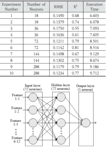
Given the dataset, it was necessary to define a basic neural network topology to conduct an experiment. In our work, this consisted of one input layer, two hidden layers, and one output layer, in which the number of neurons had to be set. The number of neurons in the input layer was set to 12 and the number in the output layer was set to one.
To determine the number of neurons in the hidden layers, an experiment was conducted in which the root mean square errors RMSE[7][8], R2(R square) and the execution time were measured for various numbers of neurons. The results are listed in Table 2.
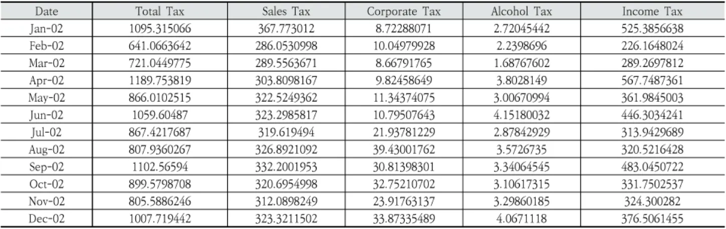
Date Total Tax Sales Tax Corporate Tax Alcohol Tax Income Tax
Jan-02 1095.315066 367.773012 8.72288071 2.72045442 525.3856638
Feb-02 641.0663642 286.0530998 10.04979928 2.2398696 226.1648024
Mar-02 721.0449775 289.5563671 8.66791765 1.68767602 289.2697812
Apr-02 1189.753819 303.8098167 9.82458649 3.8028149 567.7487361
May-02 866.0102515 322.5249362 11.34374075 3.00670994 361.9845003
Jun-02 1059.60487 323.2985817 10.79507643 4.15180032 446.3034241
Jul-02 867.4217687 319.619494 21.93781229 2.87842929 313.9429689
Aug-02 807.9360267 326.8921092 39.43001762 3.5726735 320.5216428
Sep-02 1102.56594 332.2001953 30.81398301 3.34064545 483.0450722
Oct-02 899.5798708 320.6954998 32.75210702 3.10617315 331.7502537
Nov-02 805.5886246 312.0898249 23.91763137 3.29860185 324.300282
Dec-02 1007.719442 323.3211502 33.87335489 4.0671118 376.5061455
Table 1. Structure of a Part of the Dataset used in the Experiment. The Values are in Millions of United States (U.S.) Dollars
From the results, we can see that the experiments with 72 neurons had the lowest error along with highest R-squared score and that the execution time increased with the number of neurons. Therefore, increasing the number of neurons did not necessarily provide better results. Correspondingly, we set the number of neurons in the hidden layers to 72. The final topology is illustrated in Fig. 1.
3.3 Experimental Method
This experiment was carried out in Jupyter Notebook with Python as the programming language.
The entire method of the experiment is illustrated in Fig. 2, which consists of nine steps:
Step 1. The dataset was imported to train a specific neural network. The original data were stored in a comma separated value (CSV) format in an external file. The data were then converted into a data frame object to conveniently correct missing data and reshape the data. The “read.csv” function provided by the pandas library was used to handle these objects [11].
Step 2. The original dataset was scaled. The dataset had six different features, and each feature had a different range of values, which could lead to an increased loss in training and testing. Therefore, it was necessary to convert all the data values into values of the same scale. An advantage of scaling is that it can increase the calculation speed, as the calculation becomes easier after scaling. The scaling of the dataset was done using a MinMaxScaler function in the scikit-learn library [12].
Step 3. The features were rearranged, input/output data were identified, and the decision was made about what information would be fed to the algorithm and what the expected outcome would be.
This dataset was of a supervised form. One of the important properties of financial time series data is that they yield similar trends every 12 months based on a 12-month seasonality. This property can be used to improve the training performance. Therefore, data from the previous 12 months were used as the input and output data for training specific models.
In the original dataset, there was one value of total tax and monthly tax data. Thus, it contained 72 input features and one output after the conversion of the data into the supervised form. This conversion can be done manually in Excel using the simple
“shift” function, which moves the input features of a desired number of rows into a single row at the output.
Step 4. The data in supervised form were split into training and test datasets. The training dataset was used for training the neural network and contained all the outputs against the corresponding inputs. The defined neural network utilized this data to generate Fig. 2. Performance Evaluation Processes by Building Nerual
Network Model for Each Algorithm
Fig. 1. Artificial Neural Network Structure to Compare Each Algorithm in the Experiment
Experiment Number
Number of
Neurons RMSE R2 Execution Time
1 18 0.1490 0.68 6.603
2 18 0.1379 0.74 6.078
3 36 0.1750 0.55 7.093
4 36 0.1636 0.61 7.605
5 72 0.1211 0.79 8.501
6 72 0.1142 0.81 8.516
7 144 0.1498 0.67 9.129
8 144 0.1302 0.75 8.674
9 288 0.1179 0.79 9.186
10 288 0.1234 0.77 9.712
Table 2. RMSE and Execution Time According to the Number of Neurons
appropriate weights to be used for making pre- dictions. The test dataset was used to evaluate the performance of a defined neural network after it had been trained. The test dataset did not contain the output so that the neural network could be properly tested. Predictions were made using the trained neural network with the test dataset, and the results were compared with the actual values to evaluate the network. The dataset was split so that 180 rows were used as the training dataset and the last 12 rows were used as the test dataset. The general rule is to use around 20% data for test purpose but due small data size, more data was given to model for training purpose.
Step 5. The hyperparameters were set before training the neural network. Hyperparameters define high-level concepts, such as the complexity of the model and its capacity to learn, and they must be defined manually. The only way to find optimal values is to set different values, train the models, and choose those values that produce the best results.
The hyperparameters that were set in this experi- ment included the number of hidden layers, the number of nodes in the hidden layers, the activation function, and the optimizer. Hidden layers were created between the input and output layers to increase the performance of the model. When the number of hidden layers is decided, certain aspects of the model should be considered. First, it should be determined whether a deep or shallow model is to be used. If a shallow type is chosen there would be no hidden layers only the input and output layers.
Otherwise, it will be more than two. Next, the complexity of the data should be considered. If the data are very complex, a deep network would be more suitable than a shallow one to provide correct predictions. However, some research shows that the number of hidden layers has no effect on the learning abilities of a neural network beyond a certain number [13,14]. Therefore, we have to identify this number, which can be achieved by assessing different configurations, evaluating the performance, and choosing the one with the best outcomes. After the determination of the number of hidden layers, the number of nodes should be determined. A node takes weighted inputs from the training set or previous layer, applies an activation function, and generates the output. The general operation of a node can be summed up in the form of the Equation (1).
′ ∗ (1)
In the equation, x’ is the output of the neuron, x is the input to the neuron, T is the weight assigned to the input, B is the bias, and A is the activation function.
The number of nodes has a tradeoff relationship with the processing time in a model, because a node is a computational unit. There is no limit on the number of neurons in a single layer and there can be few or many neurons. However, the only way to determine the ideal number of nodes is to test different numbers and to choose the one with the shorter processing time and the better performance.
Subsequently, the activation function needs to be decided. For the hidden layer, a rectified linear unit (ReLu) function was used, and for the output layer, a simple linear activation function was used [15,16].
The last parameter we set was an optimizer. The extensively used optimization algorithms for data prediction neural networks are Adam [17], RMSprop, stochastic gradient descent (SGD), and Adagrad [18].
We conducted experiments with all four optimizers in each tested neural network.
Step 6. The four machine learning models were built using libraries provided by Keras and TensorFlow [19][20]. Each model had the same number of hidden layers and the same number of nodes in each hidden layer. Additionally, the same activation function and optimizer were used in the comparison experiment.
The basic ANN model had one hidden layer that comprised dense layers. The dense layer are fully connected to each node on all layers in a neural network. Fig. 3 shows the program sample code to define the model.
The RNN model also had one hidden layer, and its hidden layer was made up of simple RNN units. The RNN units were more complicated than basic neurons because they contained feedback loops to retain additional information and to achieve better results. Fig. 4 shows the program code used to define the RNN model.
The LSTM is the most advanced form of a recurrent neural network to date. It achieves accurate results in different situations. As the name suggests, this model is capable of having a very long memory and can increase the chances of better results. The design of the LSTM model differs only in the hidden layer, which consists of LSTM units [24]. Fig. 5 represents a sample of the source code to define an
LSTM neural network model.
Step 7. The models were compiled, and the loss function was set to calculate errors to evaluate the trained models. In most learning networks, the error is calculated as the difference between the actual output y and the predicted output ŷ. The function that is used to compute this error is known as the loss or cost function. The loss function used in this experiment was the RMSE [22], which is extensively used in linear regression as the performance measure.
To calculate the RMSE, Equation (2) was used:
RMSEmi m ∥yi yi ∥ (2)
where y(i) is the actual expected output, and ŷ(i) is the prediction of the model. Also, m is the number of datasets. To minimize the loss function, the model parameters were periodically updated by an optimizer.
The optimizer changes the parameters and minimizes the errors of the loss function as soon as possible to avoid high computation costs and to provide better results.
In this experiment, the Adam optimizer was used.
Step 8. The compiled model was fitted using the training data. A fitting method was used to learn the parameters from the training data, and a transform method was used with those parameters to make
predictions on the test data. If the calculated RMSE was higher than a threshold value of loss, the model was trained again after changing hyper-parameters to reduce the loss. The meaning of hyper-parameters are initial values for training and testing that include activation function, initial weights, kind of optimizer. For example, activation functions that can be applied are sigmoid function, rectified unit (ReLu), and step function.
The program was executed multiple times to set the optimal parameters to achieve the best results.
Step 9. Each algorithm was evaluated by measuring the RMSE, R2 and the processing times. R-squared is a statistical metrics that represents the proportion of variance for a dependent variable that’s explained by an independent variable or variables in a regression model. Furthermore, future total taxes were predicted using each model, and the results were compared to the recorded taxes. The source code used for predictions is illustrated in Fig. 6.
To perform the prediction, input data were acquired from the test data. A comparison between the real tax values and predicted ones is shown in Fig. 7.
The hardware specifications for this experimental environment were as follows. The central processing unit (CPU) used was a 2.4 GHz dual-core Intel i7 CPU, and the memory was a double data rate 3 (DDR3) equal to 8 GB with a bandwidth of 1600 MHz The graphics card used was Intel Iris 1536 MB Graphics.
4. Results
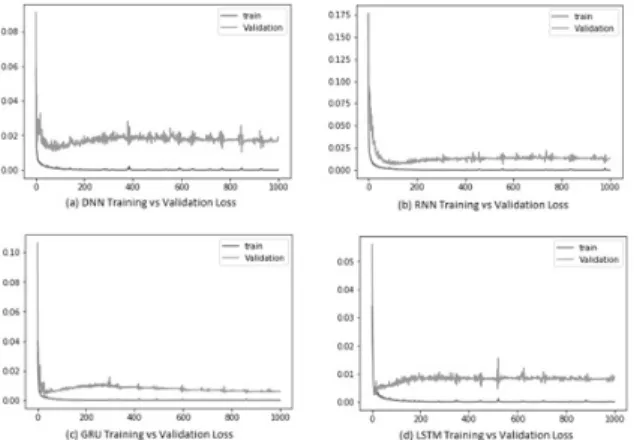
In this section, the experimental results are discussed for each network model. First, the trends of the training and validation losses are compared among the neural network models. In this experiment, the Adam optimizer was used, the ReLu activation function was used, the number of epochs was set to 500, and the number of neurons in the hidden layers was set to 72. The results are presented in Fig. 8.
From Fig. 8, we can see that the training losses converged at similar rates, but the validation losses converged at different rates. As expected, the simple DNN yielded the minimum convergence in the training loss when compared to the other schemes, because its structure did not have the necessary complexity to train a model. The other schemes were based on RNNs. Hence, their validation loss Fig. 4. An Example of the Source Code to Define an RNN Model
Fig. 5. An Example of the Source Code used to Define an LSTM Neural Network Model
Fig. 3. An Example of the Source Code to Define the Basic Artificial Neural Network Model
decreased at similar rates; however, there were some differences among them. The trend of the validation loss in the pure RNN decreased in a more stable manner than that of the GRU or the LSTM. Additionally, over-fitting did not occur. In the case of the GRU, the validation loss increased slightly at the beginning of the iterations, but it finally converged and fit the dataset well. After 1000 iterations, the GRU exhibited better performance than the pure RNN and the LSTM. In the LSTM, the validation loss showed a similar pattern to that of the GRU, and a much higher loss than the training loss at the beginning of the iterations. This occurred because the model was not trained adequately to achieve good prediction accuracies, owing to insufficient data. As the iterations progressed, the algorithm updated its weights based on the training data. Once the algorithm reached a global minimum, it stopped updating the weights and the loss graph remained unchanged. If an algorithm is tuned well, almost all machine learning algorithms exhibit similar patterns. Accordingly, the validation loss is increased at the beginning, and when the number of iterations increases, the validation loss decreases. In Fig. 8, the graphs of the LSTM and the GRU are almost identical to each other. This is owing to their similar nature: the GRU is a simpler version of the LSTM. Therefore, if the data are not
very complex, both the GRU and the LSTM will show quite similar results.
Second, the algorithms were compared based on the measured losses and processing times. In this experiment, hyperparameters of the same value were set for each algorithm. Table 3 represents the experimental results for each model.
As can be observed from the results, the DNN achieved the worst performance, as measured by RMSE. This is because it used a basic back-propagation neural network with a simple architecture. In deep learning, if a simple neural network is used with complex input data, then it is difficult to achieve good results.
Furthermore, the DNN yielded the highest RMSE, owing to the data from a time series dataset.
An interesting result in this experiment was that the GRU and the LSTM achieved similar results in every trial. However, the GRU outperformed the LSTM in most trials for a few reasons. One is that our dataset was not very large. In general, GRUs are known to be more effective with smaller datasets compared with LSTMs. The second reason is that the LSTM is most efficiently used to remember long sequences of data, whereas in our experiment, the sequence only comprised 12-time steps [23][24].
Finally, we believe that the LSTM is too complex for this dataset. This explains why the outcome is worse than expected.
From Table 3, it can be observed that the DNN required the shortest processing time, while the LSTM required the longest processing time. This is expected, given that DNNs are structurally the most simple and lightweight, whereas LSTMs are the most complex. In the last and final experiment, the LSTM Fig. 8. Comparison of Variations of Training and Validation
Losses for Each Scheme Fig. 6. An Example of the Source Code used to Predict
Future Tax Revenue using a Trained RNN
Fig. 7. Visualization of a Comparison between the Predicted and Actual Taxes (100 Million USD) with a Trained RNN Model
yielded better results than the GRU, but required a considerable amount of time for processing. The tradeoff between the processing time and the performance is not worth it.
Third, the effect of the activation function was analyzed by comparing the RMSE errors and the processing times for all models using tanh or ReLU as the activation function. ReLU and tanh are the two most extensively used activation functions [26]. Specifically, tanh converts the original data values into a range from –1 to 1, whereas ReLU has a range of from 0 to infinity. In this experiment, the Adam optimizer was used. Table 4 lists the results for each model.
The results show that the RNN-based algorithms, i.e., RNN, GRU, and LSTM, are improved when the ReLU is used rather than when tanh is used. For example, the RMSE value of LSTM with ReLU is 0.0854 and with tanh is 0.1732. The value with tanh is almost twice than the value with ReLU. The reason for this is that the converted values produced by tanh have negative range numbers, and our data consisted of positive values. The processing time with ReLU is slightly longer than that with tanh. This
is expected, because the ReLU algorithm is more complicated than the tanh algorithm. However, it does not require as much processing time as we expected, because it is much more complicated than tanh. Based on processing time, there was almost no difference between the activation functions in this experiment.
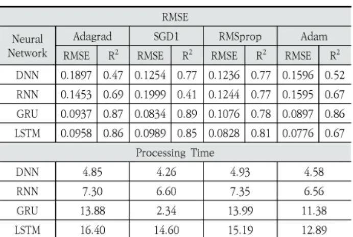
Fourth, the effect of the optimizer on the performance of each neural network model was evaluated. In this experiment, we used four optimizers: Adagrad, SGD, RMSprop, and Adam. As it can be observed from the results (Table 5), the Adam optimizer yielded the lowest RMSE for DNN, GRU, and LSTM. The reason for this is that it uses adaptive moment estimation and past gradients to calculate the current gradients.
The Adam optimizer also utilizes the concept of momentum by adding fractions of previous gradients to the current one. This optimizer has become widespread and is practically accepted for use in training neural networks. For the basic RNN, RMSprop shows the best performance for RMSE errors.
SGD, stochastic gradient descent; DNN, deep neural network; RNN, recurrent neural network; GRU, gated recurrent unit; LSTM, long short-term memory; RMSE, root mean square error.
However, the Adam optimizer yields the worst performance regarding processing time, irrespective of the algorithm. The reason for this is that it takes a long time for the optimizer to identify the global minimum cost for the problem. Furthermore, this is attributed to the increased complexity of the algorithm. This means that it always yields a solution with the lowest possible cost. In this experiment, we can observe that the loss exhibits a tradeoff relationship Adam Optimizer Processing
Time (Sec) Neural
Network
Tanh ReLU
RMSE R2 RMSE R2 Tanh ReLU DNN 0.0816 0.7 0.1096 0.7 4.15 4.58 RNN 0.1146 0.67 0.0995 0.72 6.04 6.56 GRU 0.1410 0.73 0.0897 0.8 10.71 11.38 LSTM 0.1732 0.72 0.0854 0.75 12.18 12.89 Table 4. Experimental Results According to the Changing
Activation Functions of tanh and ReLU
Trials
Neural Netwok Models
Processing Time (Sec)
DNN RNN GRU LSTM
RMSE R2 RMSE R2 RMSE R2 RMSE R2 DNN RNN GRU LSTM 1 0.12 0.47 0.14 0.69 0.10 0.87 0.11 0.86 4.27 6.06 10.91 12.52 2 0.15 0.82 0.21 0.63 0.08 0.83 0.09 0.65 4.16 6.05 10.82 12.34 3 0.15 0.76 0.16 0.87 0.13 0.74 0.13 0.64 4.21 6.11 10.79 12.25 4 0.23 0.34 0.18 0.58 0.14 0.77 0.13 0.76 4.19 6.14 10.82 12.41 5 0.14 0.73 0.15 0.73 0.12 0.78 0.13 0.85 4.22 6.47 11.15 12.37 6 0.16 0.69 0.15 0.78 0.10 0.76 0.11 0.83 4.19 6.07 10.84 12.21 7 0.18 0.48 0.10 0.8 0.13 0.87 0.13 0.75 4.20 6.09 10.81 12.25 8 0.18 0.6 0.17 0.71 0.10 0.71 0.12 0.72 4.28 6.06 10.83 12.27 9 0.10 0.71 0.13 0.69 0.15 0.74 0.11 0.71 4.23 6.11 10.98 12.46 10 0.17 0.7 0.11 0.72 0.12 0.82 0.12 0.75 4.22 6.07 11.18 12.84 Avg 0.16 0.63 0.15 0.72 0.12 0.78 0.12 0.75 4.21 6.12 10.91 12.38
Table 3. Experimental Results : RMSE, R2, and Processing Time
RMSE Neural
Network
Adagrad SGD1 RMSprop Adam
RMSE R2 RMSE R2 RMSE R2 RMSE R2 DNN 0.1897 0.47 0.1254 0.77 0.1236 0.77 0.1596 0.52 RNN 0.1453 0.69 0.1999 0.41 0.1244 0.77 0.1595 0.67 GRU 0.0937 0.87 0.0834 0.89 0.1076 0.78 0.0897 0.86 LSTM 0.0958 0.86 0.0989 0.85 0.0828 0.81 0.0776 0.67
Processing Time
DNN 4.85 4.26 4.93 4.58
RNN 7.30 6.60 7.35 6.56
GRU 13.88 2.34 13.99 11.38
LSTM 16.40 14.60 15.19 12.89
Table 5. Performance Comparisons Based on the Various Optimizers
with the optimizer. Therefore, the performances of the optimizers are not based on a simple reason.
There are many unknown variables, such as the weights, that can affect the performances of the optimizers. An optimizer may perform well in one experiment and worse in another one. The only way to select an optimizer is to test all of them and then decide based on the results.
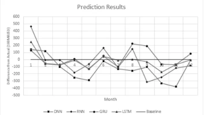
Fifth, the total taxes for the upcoming 12 months were predicted with the four trained neural network models. The resulting tax revenues were compared to the observed total taxes. Fig. 9 shows the pre- dicted results of each scheme. The solid line shows the actual values, whereas the dotted line graphs represent the total values predicted by each neural network model. From Fig. 9, it can be observed that the LSTM and GRU achieved the best performances among all of the tested models.
The DNN model achieved good predictions in the first two months. Subsequently, the accuracy decreased gradually compared to that of the other models. This is attributed to the simple structure of the DNN, which does not consider uncertainties or past patterns. All of the other algorithms yielded improved performances compared to the DNN because they utilized previous values and time steps for future tax predictions. Among the recurrent algorithms, the RNN achieved the worse performance in comparison to the GRU and LSTM. The reason for this is that it still has a vanishing gradient problem. Both the GRU and LSTM yielded prediction outcomes, and the values of the LSTM were closer to most of the actual values.
This is attributed to the fact that the LSTM retains useful information from long sequences in time series data that is subsequently used for predictions.
To evaluate the contribution of the research qualitatively, it was compared with the previous research. The recent research related to machine learning algorithm comparison can be found in [19].
In this research, they have compared random forest algorithm, k-nearest neighbor (KNN) algorithm, and scalable vector machine (SVM) algorithm to find the best performance model for predicting crime hotspot.
When compared with this, our research has the following benefits. First, the previous research did not compared the effects of the hyper-parameters while these are very important factors of the performance. Our researches presented the effects clearly. Second. they did not compare the execution time taken to train neural network models. The learning time is one of the important factors to be considered when choosing algorithm. Third, they did not use RNN and GRU in the experiment. RNN is most widely used to predict time series data, and GRU is becoming popular. In our research, we have compared these algorithms to predict future data.
5. Conclusions
DNN, RNN, LSTM, and GRU are the most extensively used algorithms for future data prediction. However, it is not easy for developers to choose the most appropriate algorithm to use with their application because enough information on the performance of each algorithm is not available. To alleviate the difficulty, we implemented and compared the algorithms based on the evaluation of their training and test errors on a tax dataset. Furthermore, we analyzed the effects of the activation functions and optimizers on the performance of the algorithms.
For the activation function, RNN-variant algorithms yielded much better performances when ReLU was adopted compared to tanh. In the case of the optimizers, DNN, GRU, and LSTM yielded better performances when the Adam optimizer was used, and RNN achieved the best performance when RMSprop was adopted. Regarding the processing time, the Adam optimizer yielded the worst performance among all algorithms. An experiment methodology was presented to evaluate each algorithm using tax data sets. This methodology and conclusions are valuable because these also applicable to other data sets such as weather, medical, and industries.
Fig. 9. Comparison of the Future Tax Prediction Results with the Trained Models
References
[1] W. C. Wang, K. W. Chau, C. T. Cheng, and L. Qiu, “A comparison of performance of several artificial intelli- gence methods for forecasting monthly discharge time series,” Journal of Hydrology, Vol.374, No.3, pp.294-306, 2009.
[2] A. M. Logar, E. M. Corwin, and W. J. B. Oldham, “A com- parison of recurrent neural network learning algorithms,”
IEEE International Conference on Neural Networks, pp.1129-1134, 1993.
[3] A. Shrestha and A. Mahmood, “Review of deep learning algorithms and architectures,” IEEE Access, Vol.7, pp.53040-53065, 2019.
[4] S. Hochreiter and J. Schmidhuber, “Long short-term me- mory,” Neural Computation, Vol.9, No.8, pp.1735-1780, 1997.
[5] A. Sfetsos, “A comparison of various forecasting techniques applied to mean hourly wind speed time series,” Renew Energy, Vol.21, No.1, pp.23-35, 2000.
[6] C. L. Wu, K. W. Chau, and C. Fan, “Prediction of rainfall time series using modular artificial neural networks coupled with data-preprocessing techniques,” Journal of Hydrology, Vol.389, No.1, pp.146-167, 2010.
[7] G. Li and J. Shi, “On comparing three artificial neural networks for wind speed forecasting,” Applied Energy, Vol.87, No.7, pp.2313-2320, 2010.
[8] T. Chai and R. R. Draxler, “Root mean square error (RMSE) or mean absolute error (MAE)?-Arguments against avoiding RMSE in the literature,” Geoscience Model Development, Vol.7, No.3, pp.1247-1250, 2014.
[9] T. Kluyver, “Jupyter Notebooks—a publishing format for reproducible computational workflows,” Position Power Academy Publication, pp.87–90, 2016.
[10] R. Van, G. and F. L. Drake, “Python 3 Reference Manual,”
CreateSpace, 2009.
[11] G. Ariel, “pandas,” pandas-dev/pandas: Pandas.
[12] G. Varoquaux, G. Buitinck, O. Louppe, F. Grisel, Pedregosa, and A. Mueller, “Scikit-learn,” GetMobile Mobile Computu- tation. Community, Vol.19, No.1, 2015, pp.29–33.
[13] I. Shaft, J. Ahmad, S. I. Shah, and F. M. Kashif, “Impact of varying neurons and hidden layers in neural network architecture for a time frequency application,” Proceedings of the 10th IEEE International Conference on Multitopic, pp.188–193, 2006.
[14] K. Shibata and Y. Ikeda, “Effect of number of hidden neurons on learning in large-scale layered neural net- works,” Proceedings of the International Joint Conference on ICCAS-SICE, pp.5008-5013, 2009.
[15] V. Sharma and T. Avinash, “Understanding Activation Functions in Neural Networks,” Medium, Vol.4, No.12, pp.1-10, 2017.
[16] A. L. Maas, A. Y. Hannun, and A. Y. Ng, “Rectifier nonlinearities improve neural network acoustic models,”
In ICML Workshop on Deep Learning for Audio, Speech and Language Processing, Vol.28, 2013.
[17] D. P. Kingma and J. L. Ba, “Adam: A method for stochastic optimization,” Proceedings of the 3rd International Con- ference on Learning and Representation, pp.1-15, 2015.
[18] M. C. Mukkamala and M. Hein, “Variants of RMSProp and adagrad with logarithmic regret bounds,” Proceedings of the 34th International Conference on Machine Learning, Vol.5, pp.3917-3932, 2017.
[19] X. Zhang, L. Liu, L. Xiao, and J. Ji, “Comparison of Machine Learning Algorithms for Predicting Crime Hotspots,” IEEE Access, Vol.8, pp.181302-181310, 2020.
Qalab E. Abbas
https://orcid.org/000-0002-2342-4645 e-mail : [email protected]
He received a bachelor’s degree in Electrical Engineering from National University of Sciences and Technology (NUST). He is currently a master’s stu- dent at Kumoh National Institute of Technology, Gumi, South Korea. His research interests include Machine Learning, Data Processing.
Sung-Bong Jang
https://orcid.org/000-0003-3187-6585 e-mail : [email protected] He received his B.S., M.S., and Ph.D.
degrees from Korea University, Seoul, Korea in 1997, 1999, and 2010, re- spectively. He worked at the Mobile Handset R&D Center, LG Electronics from 1999 to 2012. Currently, he is an associate professor in the Department of Industry-Academy, Kumoh National Institute of Technology in Korea. His interests include Augmented Reality, Big Data Privacy, Prediction based on Artificial Neural Networks.