Measurement Feedback Control of a Class of Nonlinear Systems via Matrix Inequality Approach

Journal of Institute of Control, Robotics and Systems (2014) 20(6):631-634

http://dx.doi.org/10.5302/J.ICROS.2014.14.0031 ISSN:1976-5622 eISSN:2233-4335

행렬 부등식 접근법을 이용한 비선형 시스템의 측정 피드백 제어

Measurement Feedback Control of a Class of Nonlinear Systems via

Matrix Inequality Approach

구 민 성, 최 호 림^* (Min-Sung Koo¹ and Ho-Lim Choi^2,*)

1Department of Fire Protection Engineering, Pukyoung National University

2Department of Electrical Engineering, Dong-A University

Abstract: We propose a measurement state feedback controller for a class of nonlinear systems that have uncertain nonlinearity and sensor noise. The new design method based on the matrix inequality approach solves the measurement feedback control problem of a class of nonlinear systems. As a result, the proposed methods using a matrix inequality approach has the flexibility to apply the controller. In addition, the sensor noise can be attenuated for more generalized systems containing uncertain nonlinearities.

Keywords: measurement feedback, sensor noise, matrix inequality approach, uncertain nonlinearity

I. INTRODUCTION AND PROBLEM FORMULATION For practical systems, the measurement feedback controller with x and the sensor noise s(t) in an additive form is applied to the systems in place of the nominal controller with state x. To dilute the effect of sensor noise, there have been various control results on measurement feedback control problems [1-4,7]. The presented controller in [1,2] via high gain observer can reduce the sensor noise. In [4], using a low-pass filter for feedforward nonlinear systems, the sensor noise is reduced for the unknown magnitude, frequency, and phase. However, the considered systems and control methods in [4] are limited to a class of feedforward systems and there are other limitation such that the condition in [4] is conservative because the condition is developed based on norm-bound. In order to relax over the norm-bound condition as [6] and [9], the matrix inequality condition is presented in [3].

The goal of this paper is to present a new design method which is motivated by [3]. In this paper, the matrix inequality approach is used to solve the measurement feedback control problem of a class of nonlinear systems.

We consider the nonlinear system given by ( , , )

x&=Ax+Bu+d t x u (1) where xÎRⁿ is the state, uÎR is the input. The system matrices ( , )A B are a Brunovsky canonical pair.

The nonlinearity d( , , )t x u =[ ( , , ),d₁t x u L,d_n( , , )]t xu ^TÎRⁿ is such that d_i( , , ) :t x u R R´ ⁿ´R®R, i= L1, ,n are C ¹.

We show the conditions in [4] as follows.

Assumption 1: [4] For i=1,L,n-2, there exists a constant

0

c ³ such that

|d_i( , , ) |t x u £c x(| _i+2|+L+|x_n|+| |)u (2) where 0£a_i£a, w£w_i< ¥ and 0, £f_i£2p with the constants a>0 and w>0.

Assumption 2: [4] For i= L1, ,n, there exists a constant

i 0,

a ³ w >_i 0, and f_i such that

( ) sin( )

i i i i

s t =a w t+f (3)

where 0£a_i£a, w£w_i< ¥ and 0, £f_i£2p with the constants a>0 and w>0.

In [4], the following controller has been introduced

1/

( )( ( )) ^{kn t}

u=K e x+s t *e ^{+ e} (4)

1 2

( ) [ /1 ⁿ , , _n/ ],

K e = k e ⁺ L k e * denotes the convolution opera- tion, and s t( )=[ ( ),s t₁ L,s t_n( ]) .^T Thus, the controller (4) is equivalent to the following form.

1 1

1 1

1 1

( ) 1 0

1 0

( ( ) ( ))

( ( ) ( ))

n

n n

n i t k t

i i

n i i

n t

k t i k

i i

n i i

u k x s e d

e k x s e d

e t

e e t

t t t

e

t t t

e

- +

- -

+ +

- +

=

- +

=

= +

= +

å ò å ò

(5)

The restriction with Assumption 1 mainly comes from the fact the norm-bound condition is used. As a result, the design of the controller tends to overly conservative and less applicable to variety of nonlinearity. Next, we introduce a controller and a new matrix inequality condition on the nonlinearity, which leads to more flexibility in applying the controller.

II. MAIN RESULTS

First, we address some mathematical setups and notations.

Setups: Let A₁=[a_ij], i=1,L,n+1, j=1,L,n+1, with

Copyright© ICROS 2014

* Corresponding Author

Manuscript received March 28, 2014 / revised April 7, 2014 / accepted April 14, 2014

구민성: 부경대학교 소방공학과([email protected]) 최호림: 동아대학교 전기공학과([email protected])

※ 이 논문은 부경 대학교 자율창의학술연구비(2013년)에 의하여 연구 되었음.

구 민 성, 최 호 림 632

ij 1

a = if i= L1, , ,n j= +i 1 and a_ij=0 j¹ +i 1 B =₁ [0L , 0,1]^T is a 1 (´ n+1) vector, and K₁( )e =[ /k₁ eⁿ⁺¹,L,k_n/e²,

1/ ]

kn₊ e is a (n +1) 1´ vector. Then, A_K( )e =A₁+B K₁( ₁( ).e) Then, we define K₁=K₁(1), A_K=A_K(1). Also, we define a positive definite matrix E_e =diag[1,L,e^i-1,L,eⁿ], i = L 1, ,

1.

n + If given that A is Hurwitz, we can obtain a Lyapunov _K equation of A_K( )e ^TP( )e +P( )e A_K( )e = -e^-1E_e² with P( )ò =

E PE_窒 from A P^T_K +PA_K = - where I denotes an (I n +1)´ (n +1) identity matrix.

Notations: Throughout the paper, X denotes a 1 (´ n+1) vector as X =[ ,x x_n+1]^T and X denotes |X| [|= x₁|,L,|x_i|,

,|x_n+1|]

L for i=1,L,n+1. Also, X denotes the Euclidean norm.

From [4], set a virtual state as

1 1

1 1

1 2 0

1

( )

n n

n t

k t i k

n n i i

i

x e ^e k x t e ^{e t}dt

e

- -

+ - +

+ + -

=

=

å ò

⁽⁶⁾

From (6), we have

1

1 2

1 n

i

n n i i

i

x k x

e

+

+ + -

=

=

å

& (7)

Then, from the system (1)-(4), (6)-(7), we have ( ) 1( , , ) ( )

X& =AK e X+d t x u +q t (8) where d₁( , , )t x u =[ ( , , ),0]d t x u ^T and

1 1

2 0

1

( ) [0, ,0, ( ) ,0]

n n

k t n i t k T

n i i i

t e^e k s e ^{e t}d

q t t

e

+ - +

+ -

=

= ^L

å ò

⁽⁹⁾

Remark 1: The proposed controller (4) in [4] is composed of a scaling gain for robust control with uncertain nonlinearities and a low-pass filter for attenuating the high-frequency sensor noise. In order to analyze the steady-state behavior with the filtered measurement feedback information multi plied by a control gain, we use the virtual state (6) in [4].

Assumption 3: There exist a matrix M (ε) such that

1( , , ) ^T ( )

X E PET _{e e}d t x u £ X E M_e e E X_e (10) which plays a key role in a matrix inequality condition.

Theorem 1: (i) Select K1 such that AK are Hurwitz. (ii) Obtain P of A P^T_K +PA_K^T = - (iii) Suppose that Assumptions 2 and 3 I. hold. (iv) Suppose that there exists ² such that the following matrix inequality condition holds

1 2 ( ) 0

h窒^-I- M > (11)

with 0<h<1. Then, all states of the system (1) with the controller (4) are globally ultimately bounded.

Proof: Set V X( )=X P^T (e)X. Then, along the trajectory of (8), we have

1

( ) 2 ( ) ( , , )1

2 ( ) ( )

T T

T

V X X E E X X P t x u

X P t

e e

e e d

e q

£ - - +

+

&

(12)

By Assumption 3, we have

( ) ^T ( 1 2 ( )) 2 ^T ( ) ( )

V X& £ -X E_e e^-I- M e E X_e + X Pe q t (13) By Assumption 2, from [4], we have

1 1 2

1 2 2

1 1

| |

( ) (1 )

( / )

n n

k t

i i

n i

i n i

k a

t e

k w

q e

e e

- + + -

= +

£ +

å

+ ⁽¹⁴⁾

Using (14), we have

1 1 1

1

3 2 2

1 1

( ) ( ) ( )

| |

(1 )

( / )

n

T n

n

k t

i i

i

i n i

X P t P E X t

k a

e

k w

P E X

e

e

e

e q e q

e e

- + -

-

= +

£

æ ö

ç ÷

£ +

ç + ÷

è ø

´

å

⁽¹⁵⁾

From (13) and (15), we have

1

1

( ) ( 2 ( ))

((1 ) ( ))

V X X E hT I M E X

E X h E X

e e

e e

e e

e s e

-

-

£ - -

- - -

&

(16)

where ₃ ^{1 1}

2 2

1 1

| |

( ) (1 )

( /

. )

n n

k t

i i

i

i n i

k a

e P

k w

s e e

e e

- + -

= +

æ ö

ç ÷

= +

ç + ÷

è ø

å

Dut to k_n+1<0, ₃

2 2

1 1

| |

( ) 0

( / )

n

i i

i

i n i

k a

P

k w

s e ⁼ e ^- ₊ e

æ ö

ç ÷

® <

ç + ÷

è ø

å

^as

.

t ® ¥ From (16), it is obvious that there exists a positive constant b such that ^* E X_e £b^* as t ® ¥ for any X(0) because V X £&( ) 0 when E X_e ³s e( ). Thus, E X_e is globally ultimately bounded from (11) and (16) from [5]. Then, it is obvious that x is globally ultimately bounded.

In the following example, we illustrate the construction of ( ).

M e

Example A: Consider the following system

2

2 1

1 2

2

2

sin 1 10

x x

x x

x

x u

= +

+

=

&

&

(17)

Suppose that there exists a nonzero measurement noise s t ₁( ) and s t =₂( ) 0. The existing control methods in [1-4,6-9] are not applicable to the system (17). Select K = - - -₁ [ 1, 3, 3]. From (4), we have

3 1 3 3

3 3 0 1 2 0 2

1 3

( ) ( )

t t

u x e ^e t s t e d^t t s t e d^t t

e e

- - æ ö

= + ç- - ÷

è

ò ò

ø ⁽¹⁸⁾

where

3 1 3 3

3 3 0 1 2 0 2

1 3

( ) ( )

t t

x e ^e t x t e d^t t x t e d^t t

e e

- - æ ö

= ç- - ÷

è

ò ò

ø ⁽¹⁹⁾

and x&₃=K₁( ) .e X

Then, we have

2.3125 1.9375 0.5000 1.9375 3.2500 0.8125

0.5000 0.8125 5

. 0.437 P

é ù

ê ú

=ê ú

ê ú

ë û

Min-Sung Koo and Ho-Lim Choi

행렬 부등식 접근법을 이용한 비선형 시스템의 측정 피드백 제어 633

From Assumption 3, using

2

2 1

2 2

sin 0.1

1 1 ,

0

x x

x £ x

+ we obtain

2

2 1

1

2

2 2

1

2

3 2

2

( , , ) sin 0 0

1 10

0.1(2.3125 1.9375 0.5000 )

( )

T T

T

x x

X E PE t x u X E P x

x x x x x

X E M E X

e e e

e e

d

e e

e

é ù

= ê ú

ê + ú

ë û

£ + +

=

(20)

where

1

0 2.3125 0

( ) 0.05 2.3125 3.8750 0.5000

0 0.5000 0

M e e^-

é ù

ê ú

= ê ú

ê ú

ë û

(21)

Then, from the condition (11) in Theorem 1, it is obvious That

1 2 ( ) 0

he^-I- M e > with h =0.5 for any e>0.

Lemma 1: If Assumption 1 holds. Then, Assumption 3 holds, not vice versa.

Proof: Note that

1 2

1 1

| ( , , ) | | |

n n

i

i i

i i

t x u c x

e^- d e^-

= =

å

£

å

⁽²²⁾

Then, it is clear from Lemma 1 in [3].

III. APPLICATION EXAMPLE We consider the inertial wheel pendulum [8]

1 2 0 1 1 2 2

2 3

3

sin

x x m m x m x

x x

x u

= + +

=

=

&

&

&

(23)

where m £₀ 0.01, m £₁ 1, and m £₂ 0.01. Suppose that there exists a nonzero measurement noise s t and ₁( ) s t₂( )=s t₃( )=0.

For new features, only the bound of the parameters m₂ is known.

Due to the term m₀sinm x_{1 1}+m x_{2 2} and the noise s t the ₁( ), existing controllers in [1-4,6-9] can not be applicable to the system (23).

Select K = - - - -₁ [ 1, 4, 6, 4]. From (4), we have

4 1 4 4

4 4 0 1 3 0 2

4 2 0 3

1 6

( ) ( )

4 ( )

t t

t

t

u x e s e d s e d

s e d

e t t

t

t t t t

e e

t t

e

- - æ

= + ç- -

è

- ö÷

ø

ò ò

ò

(24)

where

4 1 4 4

4 4 0 1 3 0 2

4 2 0 3

1 6

( ) ( )

4 ( )

t t

t

t

x e x e d x e d

x e d

e t t

t

t t t t

e e

t t

e

- - æ

= ç- -

è

- ö÷

ø

ò ò

ò

(25)

and x&₄=K₁( ) .e X

Then, we have

3.1250 4.0000 2.3750 0.5000 4.0000 8.3750 5.5000 1.1250 2.3750 5.5000 5.1250 1.0000 0.5000 1.1250 1.0000 0. 0 . 375 P

é ù

ê ú

ê ú

=ê ú

ê ú

ê ú

ë û

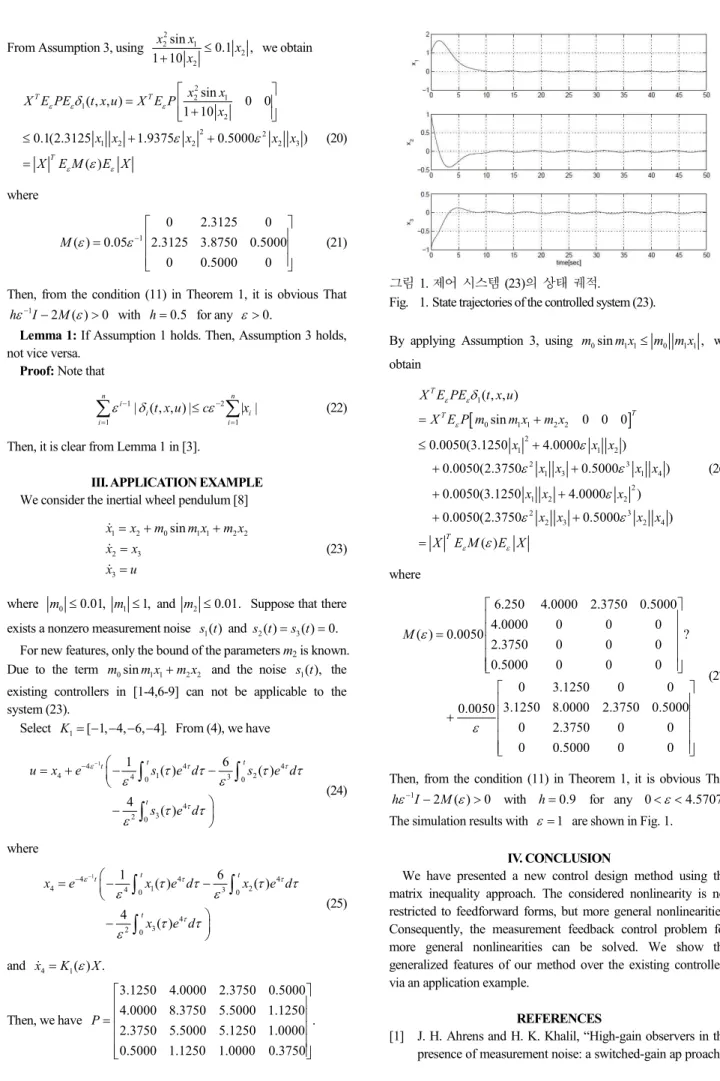
그림 1. 제어 시스템 (23)의 상태 궤적.

Fig. 1. State trajectories of the controlled system (23).

By applying Assumption 3, using m₀sinm x_{1 1}£ m m x_{0 1 1}, we obtain

[ ]

2

3 1

0 1 1 2 2

2

1 1

2 3

1 1

2 4

2 2

2 3 2 4

1

2 3

( , , )

sin 0 0 0

0.0050(3.1250 4.0000 )

0.0050(2.3750 0.5000 )

0.0050(3.1250 4.0000 )

0.0050(2.3750 0.5000 )

) (

T

T T

T

X E PE t x u

X E P m m x m x

x x x

x x x x

x x x

x x x x

X E M E X

e e

e

e e

d

e

e e

e

e e

e

= +

£ +

+ +

+ +

+ +

=

(26)

where

6.250 4.0000 2.3750 0.5000

4.0000 0 0 0

( ) 0.0050 ?

2.3750 0 0 0

0.5000 0 0 0

0 3.1250 0 0

3.1250 8.0000 2.3750 0.5000 0.0050

0 2.3750 0 0

0 0.5000 0 0

M e

e

é ù

ê ú

ê ú

= ê ú

ê ú

ê ú

ë û

é ù

ê ú

ê ú

+ ê ú

ê ú

ê ú

ë û

(27)

Then, from the condition (11) in Theorem 1, it is obvious That

1 2 ( ) 0

he^-I- M e > with h =0.9 for any 0<e<4.5707. The simulation results with e= are shown in Fig. 1. 1

IV. CONCLUSION

We have presented a new control design method using the matrix inequality approach. The considered nonlinearity is not restricted to feedforward forms, but more general nonlinearities.

Consequently, the measurement feedback control problem for more general nonlinearities can be solved. We show the generalized features of our method over the existing controllers via an application example.

REFERENCES

[1] J. H. Ahrens and H. K. Khalil, “High-gain observers in the presence of measurement noise: a switched-gain ap proach,”

Measurement Feedback Control of a Class of Nonlinear Systems via Matrix Inequality Approach

구 민 성, 최 호 림 634

Automatica, vol. 45, no. 4, pp. 936-943, 2009.

[2] A. A. Ball and H. K. Khalil, “High-gain observers in the presence of measurement noise: a nonlinear gain approach,”

Proceedings of the 47th IEEE Conference on Decision and Control, Cancun, Mexico, pp. 2288-2293, Dec. 2008.

[3] Z. Chen, “Improved controller design on robust appoximate feedback linearization via LMI approach,” IEICE Trans.

Fundamentals, vol. E88-A, no. 7, pp. 2023-2025, 2005.

[4] H.-W. Jo, H.-L. Choi, and J.-T. Lim, “Measurement feedback control for a class of feedforward nonlinear systems,” International Journal of Robust and Nonlinear Control, vol. 23, no. 12, pp. 1405-1418, 2013.

[5] H. K. Khalil, Nonlinear Systems, 3rd ed., Prentice Hall, Upper Saddle River, NJ 07458, 2002.

[6] H. Lei and W. Lin, “Universal adaptive control of nonlinear systems with unknown growth rate by output feedback,”

Automatica, vol. 42, no. 10, pp. 1783-1789, 2006.

[7] J. P. Jiang, I. Mareels, and D. Hill, “Robust control of uncertain nonlinear systems via measurement feedback,”

IEEE Transactions on Automatic Control, vol. 44, no. 4, pp.

807-812, 1999.

[8] R. Olfari-Saber, Nonlinear Control of Underactuated Mechanical Systems with Application to Robotics and Aerospace Vehicles, Ph.D. Dissertation, MIT, 2001.

[9] X. Ye and H. Unbehauen, “Global adaptive stabilization for a class of feedforward nonlinear systems,” IEEE Trans. on Automat. Contr., vol. 49, no. 5, pp. 786-792, 2004.

구 민 성

received the B.S.E. degree in 2004 and M.S.

degree in 2006 and Ph.D. degree in 2011 from the department of electrical engineering, KAIST (Korea Advanced Institute of Science and Technology), Daejeon, Korea, respectively.

She is an assistant professor at the department of Fire Protection Engineering, Pukyong National University, Busan. Her research interests include nonlinear system, delay system, high-order system.

최 호 림

제어·로봇·시스템학회 논문지 제15권 제6호 참조.