1. INTRODUCTION
Animal recognition and classification have been considered as the forefront topic of computer vision.
The problem with the automatic system is that, Animals do not appear individually at a scene rath- er it takes all the natural objects around it.
Therefore, for the computer, it has to rectify the animal figure first and then classify it where hu-
mans can easily concentrate only on the animal.
Besides, animals may appear under different illu- mination conditions, viewpoints, scales and shapes [1]. Methods for classifying human faces have been established with great accuracy but for the animal classifications, those methods have been proved far from accurate because of the diversity of animal classes with complex intra-class variability and inter-class similarity [1]. Researchers have at-
Animal Face Classification using Dual Deep Convolutional Neural Network
Rafiul Hasan Khan
†, Kyung-Won Kang
††, Seon-Ja Lim
†††, Sung-Dae Youn
††††, Oh-Jun Kwon
†††††, Suk-Hwan Lee
††††††, Ki-Ryong Kwon
†††††††ABSTRACT
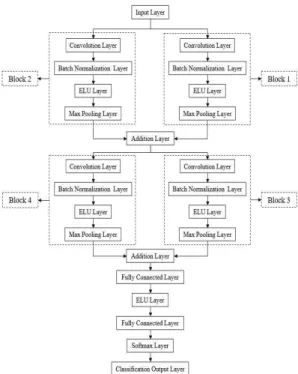
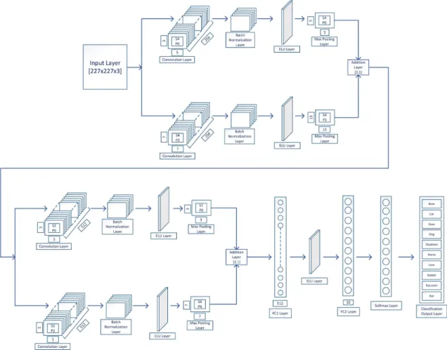
A practical animal face classification system that classifies animals in image and video data is considered as a pivotal topic in machine learning. In this research, we are proposing a novel method of fully connected dual Deep Convolutional Neural Network (DCNN), which extracts and analyzes image features on a large scale. With the inclusion of the state of the art Batch Normalization layer and Exponential Linear Unit (ELU) layer, our proposed DCNN has gained the capability of analyzing a large amount of dataset as well as extracting more features than before. For this research, we have built our dataset containing ten thousand animal faces of ten animal classes and a dual DCNN. The significance of our network is that it has four sets of convolutional functions that work laterally with each other.
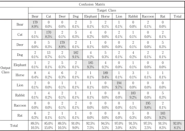
We used a relatively small amount of batch size and a large number of iteration to mitigate overfitting during the training session. We have also used image augmentation to vary the shapes of the training images for the better learning process. The results demonstrate that, with an accuracy rate of 92.0%, the proposed DCNN outruns its counterparts while causing less computing costs.
Key words: Animal Face Classification, Machine Learning, Batch Normalization, Exponential Linear Unit, Dual Deep Convolutional Neural Network.
※ Corresponding Author : Ki-Ryong Kwon, Address:
(48513) 45 Yongso-ro, Namgu, Busan, Pukyong National University, Korea, TEL : +82-51-629-6257, FAX : +82- 51-629-6230, E-mail : [email protected] Receipt date : Oct. 1, 2019, Revision date : Mar. 11, 2020 Approval date : Apr. 1, 2020
†††
Dept. of IT Convergence and Application Engineering, Pukyong National University
(E-mail : [email protected])
†††
Dept. of Information and Communication Engineering, Tongmyong University (E-mail : [email protected])
†††
Dept. of Computer Engineering, Pukyong National University (E-mail : [email protected])
†††††††
Dept. of Computer Engineering, Pukyong National University (E-mail : [email protected])
†††††††
Dept. of Computer Software Engineering, Dongeui University (E-mail : [email protected])
†††††††
Dept. of Computer Engineering, Dong-A University (E-mail : [email protected])
†††††††
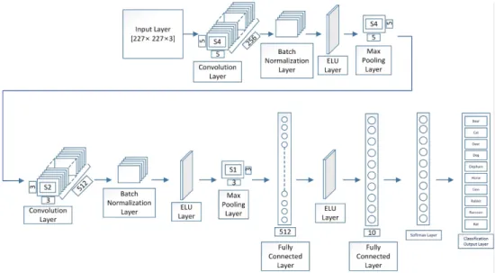
![Fig. 2. The DCNN of Tibor Trnovszky et al. [5].](https://thumb-ap.123doks.com/thumbv2/123dokinfo/4755995.515874/4.807.144.665.786.989/fig-dcnn-tibor-trnovszky-et-al.webp)