Estimation of Suitable Methodology for Determining Weibull Parameters for the Vortex Shedding Analysis of Synovial Fluid

학 술 논 문

21

Estimation of Suitable Methodology for Determining Weibull Parameters for the Vortex Shedding Analysis of Synovial Fluid

Nishant Kumar Singh, A. Sarkar

, Anandita Deo, Kirti Gautam and S.K Rai

School of Biomedical Engineering, Indian Institute of Technology, (Banaras Hindu University), Varanasi, India

1

Department of Mechanical Engineering, Indian Institute of Technology, (Banaras Hindu University), Varanasi, India

(Manuscript received 18 November 2015; revised 28 December 2015; accepted 29 December 2015)

Abstract: Weibull distribution with two parameters, shape (k) and scale (s) parameters are used to model the fatigue failure analysis due to periodic vortex shedding of the synovial fluid in knee joints. In order to determine the later parameter, a suitable statistical model is required for velocity distribution of synovial fluid flow. Hence, wide appli- cability of Weibull distribution in life testing and reliability analysis can be applied to describe the probability dis- tribution of synovial fluid flow velocity. In this work, comparisons of three most widely used methods for estimating Weibull parameters are carried out; i.e. the least square estimation method (LSEM), maximum likelihood estimator (MLE) and the method of moment (MOM), to study fatigue failure of bone joint due to periodic vortex shedding of synovial fluid. The performances of these methods are compared through the analysis of computer generated synovial fluidflow velocity distribution in the physiological range. Significant values for the (k) and (s) parameters are obtained by comparing these methods. The criterions such as root mean square error (RMSE), coefficient of determination (R

), maximum error between the cumulative distribution functions (CDFs) or Kolmogorov-Smirnov (K-S) and the chi square tests are used for the comparison of the suitability of these methods. The results show that maximum likelihood method performs well for most of the cases studied and hence recommended.

Key words: Weibull distribution, vortex shedding, synovial fluid, least square estimation method, maximum like- lihood estimator, method of moment

I. Introduction

Synovial fluid is a plasma dialysate, which is modified by means of elements secreted by knee joint tissues that implicated in reduced friction much smaller than human made machines. The rheological premises of synovial fluid sound to be particularly suited for joint lubrication [1]. In recent years, a considerable amount of work had been reported which exhibits viscoelastic properties of synovial fluid in human knee joints [2,3,4,5]. To establish the viscoelastic nature of synovial fluid, content of the same i.e. hyaluronic acid which is an essential com-

ponent, varies with age [2]. Concentration of hyaluronic acid is highest between 18 to 25 years and between the ages of 30 to 80, in normal joints no changes is observed [2,6]. Dynamic shear moduli at various strain frequencies at various temperatures show the viscoe- lastic nature of synovial fluid [7].

Balazs plotted typical set of values of the elastic and viscous moduli as a function of strain frequency from synovial fluid samples of two normal knee joints of ages 20 and 67 years and one from osteo- arthritic knee joint aged 63 years [2]. Results showed that as the strain frequency increases, both elastic and viscous moduli increase, that is different in pathological fluid considering strain frequencies in range to which the fluid was exposed in the course of normal movement of the knee joint (flexion, extension, walking and running).

However, Pekkan, Nalim and Yokota [8] predicted

Department of Mechanical Engineering, Indian Institute of Technology, (Banaras Hindu University), Varanasi, India TEL: +91-542-6702929

E-mail: [email protected]

22

shear stress induced by the synovial fluid flow on the knee joint cells and examined the oscillatory flow of Newtonian synovial fluid. Stress created due to the flow of synovial fluid during the joint motion may lead to bone degeneration and its ultimate failure.

Possible development of stress may occur if the natural frequency of the bone structure matches with the frequency of vortex shedding and the corresponding synovial flow velocity ranges can be termed as critical velocity ranges. Expected number of stress cycles in the projected working life of bone structure is related to the expected number of hours in critical flow velocity ranges.

The Weibull distribution is a one-tailed continuous probability distribution widely used in reliability and life data analysis and failure analysis of material due to its versatility [9,10]. Hence, to analyse the vortex induced vibration on the knee joint, the flow pattern of the synovial fluid is modelled using the two- parameter Weibull distribution, as there is a direct relation between the stress induced by the flow of the fluid and the velocity gradient of the synovial fluid as studied by King [11,12]. Hence, forecasting the velocity distribution of the synovial fluid flow velocities is very much important and vital. The Weibull distribu- tion function gives the probability of failure of any given specimen under test. Involved parameters i.e.

‘k’ and ‘s’ parameters have to be approximated for an offered pair of data to depict the concerned random variety of the velocity distribution set by the Weibull model.

Several numerical techniques are available to esti- mate the Weibull parameters [1,13]. Among these techniques, three are most widely used methods namely, least square estimation method (LSEM), maximum likelihood method (MLE) and method of moment (MOM). These methods are currently used to estimate the Weibull parameters in many fields of engineering that include wind speed distribution and energy applications [13,14] along with other criterions to determine the efficiency of these methods to give a precise estimate of the Weibull parameters. Different methods suit the requirement of the estimation that depends on the data set, their distribution, and the data size [14].

II. Background

Two-parameter Weibull distribution is defined by the probability density function given as:

(1)

for v > 0, where v is the velocity of synovial fluid flow,

‘k’ is the dimensionless shape parameter and ‘s’ is the scale parameter that has a dimension same as the velocity. The ‘k’ parameter determines the shape of the distribution. The ‘k’ parameter of Weibull dis- tribution is also called Weibull slope because it is the slope of the straight line of the distribution drawn in the Weibull probability paper. Larger value of k gives narrower distribution and hence a higher peak value of the curve. The cumulative distribution function (CDF) for a variable v having Weibull distribution is given by:

(2)

Cumulative probabilities are calculated by CDF, given in Eq. (2) [15].

1. Methods for estimating Weibull parameters

Three methods, widely used to estimate the Weibull parameters, are discussed briefly:

(1) Least square estimation method [LSEM]

Transformation of distribution functions of Weibull in Eq. (2) into a linear form by taking double logarithm on both the sides and rearranging as follows:

ln( −ln(1 − F(v))) = k ln v − k ln s (3) The cumulative probability, F(v) can be calculated for n samples after arranging the values of v in ascending order such that v

< v

< v

... ...v

. F(v) can be determined using the order statistics of Wilks (1948) [24] :

Substituting the parameters of F(v) evaluated by Wilks in Eq. (3), the following equation is obtained:

= k ln v − k ln s (4)

f v ( ) k s --- v

s ---

⎝ ⎠ ⎛ ⎞

v s ---

⎝ ⎠ ⎛ ⎞

⎝ – ⎠

⎛ ⎞

exp

=

F v ( ) 1 v --- s

⎝ ⎠ ⎛ ⎞

⎝ – ⎠

⎛ ⎞

exp –

=

n i – 0.7 + n 0.4 + --- ln

⎝ – ⎠

⎛ ⎞

ln

23 where, i is the rank of the velocity, which was sorted

in ascending order and n is the ensemble size. The Weibull parameters, k and s can be estimated by a straight line fitting in the plot of ln( −ln(n−i+0.7)/

(n+0.4)) verses ln v. The slope of the best-fit line gives the ‘k’ parameter.

(2) Maximum likelihood estimator [MLE]

MLE provides a direct procedure for determining Weibull parameters. The likelihood of obtaining a particular value of v is directly related to its prob- ability density function of v. Hence, Ghosh [17] and Ang et al. [18] described the likelihood of obtaining n independent observations, v

, v

, v

…, v

. To obtain parameters of Weibull distribution, equation derived by Ang et al., is transformed to get Eq. (5) and Eq.

(6) for ‘k’ and ‘s’.

(5)

(6)

Substituting Eq. (6) in Eq. (5), the following equation is obtained:

(7)

Eq. (7) was solved by Newton-Raphson iterative method to obtain the value of ‘k’. By substituting the value of k into Eq. (6), the value of ‘s’ can be deter- mined.

(3) Method of moment [MOM]

The synovial fluid velocities following Weibull dis- tribution with parameters ‘k’ and ‘s’ have mean and variance as described by Razali et al. [19]. Since, direct solutions of the equation given by Razali et al., are not obtained, solutions for equation described by him are obtained by graphical approach with modified equation given below.

(8)

where CV is the coefficient of variation defined as ,

μ and σ are the mean and standard deviation of the synovial fluid flow velocities respectively.

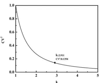
A graph of CV

verses different values of ‘k’ is plotted in MATLAB. CV

is determined by computing the mean and variance of the synovial fluid flow velocities and the corresponding ‘k’ value for the computed CV

is obtained from the graph. Fig. 1 shows the graph of CV

vs. ‘k’. Estimation of parameter ‘s’ is performed by using the equation as follows:

(9)

III. Method

The aim of this study is to determine a suitable n k

--- n – ln s + Σ

ln v Σ –

v

---- s

⎝ ⎠ ⎛ ⎞

v

---- s

⎝ ⎠ ⎛ ⎞ ln = 0

s

1 n ---Σ

v

=

n k

--- Σ

v

– n Σ

v

ln v

Σ

v

--- ln

+ = 0

CV

σ

μ

---

Γ 1 2 ⎝ ⎛ + k --- ⎠ ⎞ Γ 1 1 – ⎝ ⎛ + k --- ⎠ ⎞

Γ 1 1 ⎝ ⎛ + k --- ⎠ ⎞

---

= =

σμ---

s μ

Γ 1 1 ⎝ ⎛ + k --- ⎠ ⎞ ---

=

Fig. 1. Graph showing plot of CV

vs. k.

Fig. 2. Velocity profile of synovial fluid flow.

24

method for determining the Weibull parameters that would describe the velocity distribution of synovial fluid by considering the curve of velocity profile of synovial fluid flow as shown in Fig. 2. The range of velocity of synovial fluid during different knee motion was already determined and set to 10.00 m/s to 0.00 m/s for knee flexion and 0.00 m/s to 2.50 m/s for knee extension [20]. For the range of velocities obtained, significant values of ‘k’ and ‘s’ parameters are determined for three sets of velocities simulated by using the mean and standard deviation of the data.

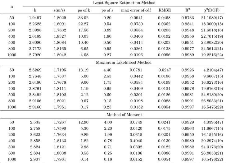
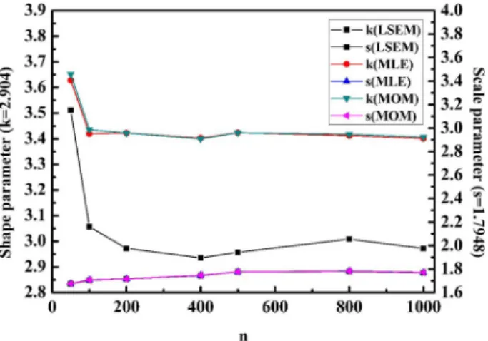
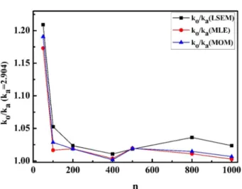
Thereafter, the two parameters of Weibull distribu- tion are determined by LSEM, MLE and MOM with sample sizes of 50, 100, 200, 400, 500, 800 and 1000.

However, data sets for velocities of synovial fluid flow are obtained by manually generated statistical algorithm in MATLAB software. This is similar to the analysis carried out by Ghosh [17], in FORTRAN program but with specified ‘k’ and ‘s’ parameters to generate random numbers, following the Weibull distribution based on the hypothesis that CDF of a continuous variable has a uniform distribution in the range 0 to 1 [22,23].

In our study, generated data must lie in the physiological range of synovial fluid flow velocity, so a random sample of 10

pseudorandom numbers are generated and uniformly distributed in the range 0 to 1. The ‘k’ and ‘s’ parameters are initially set as 2 and 4 respectively and the 10

computer generated pseudorandom numbers were treated as cumulative probabilities of the variable ‘v’. Rearranging Eq. (2) and solving for ‘v’ with the above Weibull parameters, the following equation is obtained:

(10)

The velocity values ranging from 0 to 10 m/s are selected from the generated sample to make different sets of velocities. Resulting approximate data from mean and standard deviation are treated as the actual values of ‘k’ and ‘s’. For the comparison and esti- mation of the suitability of methods, probabilities determined from Weibull function with these para- meters are treated as theoretical values, which are compared with the observed cumulative probabilities

given by the order statistics described by Wilks [24].

However, three values of ‘k’ (2.911, 2.904 and 3.37) and ‘s’ (1.773, 1.764 and 4.964) parameters are used respectively to determine the accuracy of these methods for three different sets of simulated data. The com- parisons of these three methods have been carried out by the criterions such as percent error (pe), root mean square error (RMSE), coefficient of determi- nation (R

), Komolgorov-Smirnov (K-S) test and chi square test.

(1) Goodness of fit

To determine goodness of Weibull distribution to fit the simulated data, these tests are performed at 5%

of significance level or 95% confidence interval [14].

Both K-S and chi square tests are non-parametric tests, suitable for unknown distribution and data set [15,21]. In this study, these tests are adopted to examine whether the probability distribution function with the Weibull parameters obtained from the samples (theoretical probability distribution function) is suitable to describe the synovial fluid flow velocity or not. In both the methods, comparisons of two CDFs are performed to test whether there is any significant difference between them.

K-S test determines the absolute value of the maxi- mum error between two CDFs. Critical value evaluated for K-S test at 5% significance level for one sample is as follows [14]:

(11)

The hypotheses that there is no significant difference between the two CDFs was rejected if Q > Q

. To compare the suitability of the methods, least value of Q has been considered for the better performance of test.

whereas, chi square has the form:

(12)

where, T

is the theoretical frequency of variable v determined from the CDF with specified Weibull parameters and E

is the expected frequency that can be determined from the observed probability described v s* ( – ( 1 f v – ( ) ) )

1 k---

ln

=

Q

1.36 --- n

=

χ

Σ

( T

– E

)

E

---

=

25

by order statistics of Wilks [24]. χ

gives a measure of discrepancy between the observed frequency and the expected frequency. Hence χ

= 0 shows that the two frequencies are exactly same. Larger the value of χ

represents greater difference between the observed and the expected frequencies [15]. The critical value of at α = 0.05 can be determined from the chi square distribution table for degrees of freedom n-m- 1 where n is the size of the sample or classes if data has been binned and m is the number of distribution parameters. The number of Weibull parameters in this case is 2 and hence, m = 2. Therefore, the number of degrees of freedom is n − 3. If χ

< , it was concluded that there was no significant difference between the observed and expected frequencies and the simulated velocities can be well described by theoretical Weibull distribution. To compare the suit- ability of the methods, least value of χ

was considered for the better performance of the test.

In continuation with above tests, RMSE has been considered with parameter of accuracy in CDFs. To determine RMSE, residuals are calculated by the difference between the observed probability (p

) and theoretical probability (p

). Squaring the residuals, averaging the squares, and taking the square root gives us the RMSE.

R

is also determined between the observed prob- ability and the theoretical probability to test the suitability of the methods by the following equation:

(13)

where p

is the observed probability, p

is the theor- etical probability and p

is the mean of the observed probabilities. Value of R

approaching 1 indicates that the data fitted by the theoretical distribution is well suited.

χ

χ

R

1 Σ

[ ( p

– p

)

] Σ

[ ( p

– p

)

] --- –

=

Table 1. Percent errors (pe) of Weibull parameters, RMSE and max-error in cdf between Weibull function and generated data, coefficient of determination (R

) and Chi square values with various sample size for true value of k = 2.911, s = 1.7993 m/s.

n Least Square Estimation Method

k s(m/s) pe of k pe of s max error of cdf RMSE R

χ

(DOF)

50 1.9497 1.8029 33.02 0.20 0.0941 0.0468 0.9733 21.1089(47)

100 2.2625 1.8091 22.27 0.54 0.0730 0.0362 0.9841 18.0000(15)

200 2.3998 1.7832 17.56 0.89 0.0584 0.0208 0.9948 21.6818(16)

400 2.6189 1.8327 10.03 1.80 0.0406 0.0192 0.9956 22.7015(19)

500 2.6080 1.8084 10.40 0.50 0.0414 0.0203 0.9951 23.8082(20)

800 2.7173 1.8165 6.65 0.95 0.0261 0.0138 0.9977 24.5612(21)

1000 2.7920 1.8042 4.08 0.27 0.0196 0.0096 0.9989 19.2216(22)

Maximum Likelihood Method

50 2.5269 1.7195 13.19 4.40 0.0781 0.0247 0.9926 4.2104(47)

100 2.7648 1.7537 5.00 2.53 0.0442 0.0186 0.9958 9.6667(15)

200 2.6480 1.7678 9.00 1.75 0.0584 0.0199 0.9952 16.6273(16)

400 2.8761 1.8111 1.19 0.65 0.0409 0.0134 0.9978 19.9763(19)

500 2.8492 1.8102 2.12 0.60 0.0301 0.0126 0.9981 24.8180(20)

800 2.9106 1.8021 0.07 0.15 0.0198 0.0088 0.9991 26.8053(21)

1000 2.9160 1.7951 0.17 0.23 0.0152 0.0054 0.9997 16.5476(22)

Method of Moment

50 2.535 1.7267 12.90 4.00 0.0749 0.0241 0.9929 4.0395(47)

100 2.758 1.7590 5.30 2.20 0.0420 0.0175 0.9963 11.6667(15)

200 2.623 1.7634 9.89 1.99 0.0615 0.0204 0.9950 16.1545(16)

400 2.858 1.8133 1.82 0.78 0.4040 0.0130 0.9980 20.2974(19)

500 2.824 1.8121 2.98 0.71 0.0302 0.0122 0.9982 24.3173(20)

800 2.894 1.8038 0.58 0.25 0.0196 0.0086 0.9991 26.8053(21)

1000 2.907 1.7961 0.14 0.18 0.0152 0.0054 0.9997 16.5476(22)

26

IV. Results

To analyze the performance of the three methods in estimating the Weibull parameters for vortex shedding analysis of synovial fluid, various combinations of parameter values and numbers of random variables are tested in this study. Tables 1-3, list the percent errors between the true Weibull parameters and the estimated parameters for three methods with sample size varying as 50, 100, 200, 400, 500, 800 and 1000.

The tables also list the maximum error in the CDFs, RMSE, R

and the chi square values. The critical values at 95% confidence interval in K-S and chi square tests for different sample sizes are listed in Table 4.

V. Discussions

In this current study, we reported that the maxi-

mum errors in the CDFs never exceeds the corres- ponding critical values for the K-S test implying that the theoretical Weibull distribution with its parameters estimated by different methods is appropriate to describe the observed velocity distribution.

However, the most appropriate method for deter- mining Weibull parameters can be estimated from the value of maximum error between CDFs. It has been observed that the maximum error was least in MOM followed by MLE. In Table 2, it has been observed that the value of chi square for LSEM and MOM for sample size 100 exceeded the corresponding critical value at 5% significance level. In addition, chi square value for LSEM for sample size 200 exceeded the corresponding critical value in Table 3. It implies that the theoretical model becomes inappropriate to describe the actual distribution. The MLE gave satis- factory results for all the sample sizes and various Table 2. Percent errors (pe) of Weibull parameters, RMSE and max-error in cdf between Weibull function and generated data, coefficient of determination (R

) and Chi square values with various sample size for true value of k = 2.904, s = 1.7948 m/s.

n Least Square Estimation Method

k s(m/s) pe of k pe of s max error of CDF RMSE R

χ

(DOF)

50 3.5117 1.6746 20.92 6.60 0.0799 0.0370 0.9833 6.3299(47)

100 3.0571 1.7058 5.27 4.90 0.0638 0.0282 0.9904 28.9405(14)

200 2.9725 1.7157 2.35 4.40 0.0354 0.0142 0.9976 10.2825(16)

400 2.9356 1.7444 1.08 2.80 0.0229 0.0098 0.9989 14.0711(19)

500 2.9571 1.7769 1.83 0.90 0.0218 0.0088 0.9991 15.7663(20)

800 3.0087 1.7799 3.61 0.55 0.0312 0.0133 0.9979 30.6798(21)

1000 2.9722 1.7686 2.35 1.29 0.0296 0.0129 0.9980 27.4228(22)

Maximum Likelihood Method

50 3.4069 1.6768 17.31 6.50 0.0837 0.0381 0.9823 6.9572(47)

100 2.9523 1.7081 1.66 4.80 0.0681 0.0307 0.9886 21.8571(14)

200 2.9585 1.7163 1.87 4.37 0.0362 0.0145 0.9975 8.8553(16)

400 2.9152 1.7465 1.12 2.70 0.0235 0.0094 0.9989 14.9000(19)

500 2.9611 1.7766 1.96 1.00 0.0215 0.0087 0.9991 16.5489(20)

800 2.9362 1.7837 1.10 0.60 0.0306 0.0131 0.9979 25.9900(21)

1000 2.9122 1.7711 0.28 1.30 0.0297 0.0129 0.9980 23.6791(22)

Method of Moment

50 3.4580 1.6763 19.07 6.60 0.0823 0.0376 0.9828 6.5937(47)

100 2.9870 1.7078 2.85 4.80 0.0670 0.0298 0.9892 27.5238(14)

200 2.9580 1.7160 1.85 4.40 0.0360 0.0145 0.9975 8.8553(16)

400 2.9090 1.7458 0.17 2.29 0.0229 0.0092 0.9990 14.9921(19)

500 2.9600 1.7764 1.93 1.00 0.0214 0.0087 0.9991 15.4185(20)

800 2.9470 1.7829 1.49 0.60 0.0306 0.0130 0.9980 28.7997(21)

1000 2.9240 1.7706 0.68 1.30 0.0297 0.0128 0.9980 25.1377(22)

27

degrees of freedom.

Hence, it can be stated that if the data fits the Weibull function, all the three methods are applicable to estimate the parameters, but if not, MLE per- formed the best followed by MOM.

Further, to test the suitability of LSEM, the chi square test is performed at 1% significance level. It

depicts that the calculated Chi square value did not exceed the corresponding critical value at 1% signi- ficance level. Hence, the accuracy of the method was justified. The deviation of the least square method in the chi square test for the aforementioned cases may be attributed by the randomness of the data or binning the data into classes, thus making the method less efficient for samples sizes ranging from 100 to 200.

It has been observed that the percent error obtained by LSEM are larger than those obtained by other methods with the maximum error being more than 30% in the ‘k’ parameter for sample size 50 and below. For MLE and MOM, the highest error was approximately from 12 to 13% for small sample size of 50. It proposes that the performance of least square method is worst when the sample size is smaller. The other two methods performed comparatively well even at small sample sizes with MLE giving satisfactory result in most of the cases. With the increase in the Table 3. Percent errors (pe) of Weibull parameters, RMSE and max-error in cdf between Weibull function and generated data, coefficient of determination (R

) and Chi square values with various sample size for true value of k = 3.37, s = 4.964 m/s.

n Least Square Estimation Method

K’ s’(m/s) pe of k pe of s max error of cdf RMSE R

χ

(DOF)

50 3.8395 4.7742 13.93 3.80 0.0712 0.0380 0.9824 10.7643(47)

100 4.0269 4.8069 19.49 3.20 0.0460 0.0188 0.9954 17.2500(14)

200 3.7624 4.9261 11.64 0.70 0.0486 0.0217 0.9943 31.8392(16)

400 3.4071 4.9017 1.10 1.20 0.0282 0.0098 0.9989 22.6430(19)

500 3.4673 4.9287 2.80 0.71 0.0243 0.0085 0.9991 17.8750(19)

800 3.4232 4.9267 1.60 0.75 0.0279 0.0092 0.9990 21.9099(19)

1000 3.4879 4.9855 3.50 0.40 0.0207 0.0056 0.9996 19.8328(22)

Maximum Likelihood Method

50 3.8433 4.7653 14.04 4.00 0.0068 0.0371 0.9832 10.6933(47)

100 3.9017 4.8184 15.78 2.90 0.0532 0.0191 0.9956 16.3571(14)

200 3.6527 4.9459 8.400 0.30 0.0442 0.0182 0.9960 25.1584(16)

400 3.4412 4.8933 2.100 1.40 0.0249 0.0091 0.9990 22.4509(19)

500 3.4927 4.9230 3.600 0.83 0.0220 0.0081 0.9992 20.9583(19)

800 3.4857 4.9185 3.400 0.92 0.0237 0.0084 0.9992 19.2149(19)

1000 3.4738 4.9860 3.100 0.44 0.0213 0.0057 0.9996 16.9383(22)

Method of Moment

50 3.9100 4.7654 16.02 4.00 0.0710 0.0369 0.9834 9.9640 (47)

100 3.9510 4.8154 17.24 2.90 0.0508 0.0190 0.9956 18.8095(14)

200 3.6360 4.9396 7.89 0.49 0.0419 0.0174 0.9964 26.1908(16)

400 3.4510 4.8936 2.40 1.40 0.0246 0.0091 0.9990 22.9904(19)

500 3.4980 4.9232 3.79 0.82 0.0219 0.0081 0.9992 22.7917(19)

800 3.3310 4.9302 1.15 0.68 0.0321 0.0121 0.9982 21.7507(19)

1000 3.4810 4.9856 3.30 0.43 0.0210 0.0056 0.9996 17.5114(22)

Table 4. Critical values at 95% confidence interval of Kolmogorov-Smirnov test (Q

) for various sample size n and Chi square statistics χ

(0.05) for varying degree of freedom.

n Q

Degree of freedom χ2(0.05)

50 0.192 14 23.68

100 0.136 15 25.00

200 0.096 16 26.30

400 0.068 19 30.14

500 0.0608 20 31.41

800 0.048 21 32.67

1000 0.043 22 33.92

67.50 47

28

sample size, the performance of the LSEM is improved with percent error reaching up to 3% for the sample size of 1000. For this sample size, the percent error given by MLE and MOM was reduced to 0.1 to 0.2%.

The maximum errors in the CDF obtained by LSEM are found to be larger in most of the cases, which improves with increasing data number with highest error over 8% for ‘k’. The RMSE follows the similar trend as other errors, where it decreases as the sample size increases with LSEM giving larger error than the other two methods in most of the cases.

The R

has large values for all the observations where it is approaching 1. It shows high degree of correlation between observed CDF and the CDF generated by the Weibull function using the meth- odology mentioned in Sec. 3, justifying that the techniques are suitable. It has been observed that

the R

has not much discrepancy between observations for all the three methods. The MLE performed better among all mentioned methods for determining the Weibull ‘k’ parameter. Figs. 3-5 show the estimated values of ‘k’ and ‘s’ parameters by three methods for different combinations of true values of the Weibull parameters with varying data number. The curves of estimated values of ‘k’ by MLE and MOM coincide with each other, which imply that the values esti- mated by these two methods are similar, and vary from values estimated by LSEM. The curves of esti- mated values of ‘s’ determined by three methods do not show any difference and coincide with each other.

In addition, the parameter error for Weibull ‘s’ para- meter does not show much discrepancy between different methods with the highest error being 3%. It decreases up to 0.1% as the sample size increases.

Fig. 5. Weibull shape ‘k’ and scale ‘s’ parameters calculated by different methods (k = 3.37, s = 4.964 m/s).

Fig. 6. k

/k

vs. n calculated by different methods for k

= 2.911.

Fig. 3. Weibull shape ‘k’ and scale ‘s’ parameters calculated by different methods (k = 2.911, s = 1.7993 m/s).

Fig. 4. Weibull shape ‘k’ and scale ‘s’ parameters calculated

by different methods (k = 2.904, s = 1.7948 m/s).

29

Hence, all the three methods are suitable to determine

‘s’ parameter of Weibull distribution.

However, for ‘k’ parameter error in terms of k

/k

as shown in Figs. 6-8, where k

is the observed value of ‘k’ parameter estimated by different methods with varying data number for a particular combination of

‘k’ and ‘s’ parameters and k

is the actual or targeted value of ‘k’ parameter.

It is evident that when sample size increases, observed probabilities will tend to the theoretical prob- abilities and hence the ratio will approach towards unity.

VI. Conclusions

In this paper, the performance of three methods namely LSEM, MLE and MOM for determining

Weibull parameters for vortex shedding analysis of synovial fluid has been compared. The parameters for comparison are percent error, R

, RMSE and maxi- mum error in CDF. The conclusions are drawn as follows:

(a) In simulation tests, MLE performed better followed by MOM for smaller sample sizes. The accuracy of three methods enhances as the sample size increases in most cases.

(b) MLE is rewarding for the estimation of shape parameter of the Weibull distribution.

(c) All the three methods are suitable for the esti- mation of scale parameter of Weibull distribution.

LSEM would be preferred for the ease of estimation and less percent error while determining the value of scale parameter.

References

[1] M.A. Al-Fawzan, Methods for estimating the parameters of the Weibull distribution, King Abdulaziz City for Science and Technology, Riyadh, Saudi Arabia, 2000. [Unpublished]

[2] E.A. Balazs, “Viscoelastic properties of hyaluronic acid and biological lubrication”,Univ Mich Med Cent J [Special Issue], pp. 255-259, 1968.

[3] E.A. Balazs, Some aspects of the aging and radiation sensi- tivity of the intercellular matrix with special regard to hyalu- ronic acid in synovial fluid and vitreous, Thule International Symposium: Aging of connective and skeletal tissue, Engel A and Larsson T (eds.), Stockholm: Nordiska Bokhandelns Forlag, 1969.

[4] E.A. Balazs and D.A. Gibbs, Chemistry and molecular biol- ogy of the intercellular matrix III, New York: Academic Press, 1970.

[5] E.A. Balazs and D. Watson, “Hyaluronic acid in synovial fluid. I. Molecular parameters of hyaluronic acid in normal and arthritic human fluids”, Arthritis Rheum, vol. 10, pp.

357-376, 1967.

[6] N.W. Rydell, “Decreased granulation tissue formation after installment of hyaluronic acid”, Acta Orthop Scand, vol. 41, pp. 307-311, 1970.

[7] D.A. Gibbs, E.W. Merrill, K.A. Smith and E.A. Balazs,

“Rheology of hyaluronic acid”, Biopolymers, vol. 6, pp. 777- 791, 1968.

[8] K. Pekkan, R. Nalim and H. Yokota, “Computed synovial fluid flow in a simple knee joint model”, 4th Joint Fluids Summer Engineering Conference (FEDSM), pp. 2085-2091, 2003.

[9] W. Weibull, “A statistical distribution function of wide appli- cability”, J Appl Mech-T ASME, pp. 293-297, 1951.

[10] W. Weibull, “A statistical distribution function of wide appli- cability”, J Appl Mech-T ASME, pp. 233-234, 1952.

[11] Y.C. Fung, Biomechanics, mechanical properties of living tis- sues. 2nd ed., New York: Springer-Verlag, 1993.

Fig. 7. k

/k

vs. n calculated by different methods for k

= 2.904.

Fig. 8. k

/k

vs. n calculated by different methods for k

= 3.37.

30

[12] R.G. King, “A rheological measurement of three synovial flu- ids”, Acta Rheol, vol. 5, pp. 41-44, 1966.

[13] J.V. Seguro and T.W. Lambert, “Modern estimation of the parameters of the weibull wind speed distribution for wind energy analysis”, J Wind Eng Ind Aero, vol. 85, pp. 75-84, 2000.

[14] T.P. Chang, “Performance comparison of six numerical meth- ods in estimating weibull parameters for wind energy appli- cation”, Appl Energ, vol. 88, pp. 272-282, 2011.

[15] D.C. Montgomery and G.C. Runger, Applied statistics and probability for engineers. 3rd ed., New York: John Wiley and Sons, 2003.

[16] X. Gao, J.A. Joyce and C. Roe, “An investigation of the load- ing rate dependence of the weibull stress parameters”, Eng Frac Mech, vol. 75, pp. 1451-1467, 2008.

[17] A. Ghosh, “A fortran program for fitting Weibull distribution and generating samples”, Comput Geosci, vol. 25, pp. 729- 738, 1999.

[18] A.H.-SAng and W.H. Tang, Probability concepts in engi- neering planning and design vol I: basic principles, New York: John Wiley and Sons, 1975.

[19] A.M. Razali, A.A. Salih and A.A. Mahdi, “Estimation accu- racy of weibull distribution parameters”, vol. 5, pp. 790-795, 2009.

[20] P. Pustejovska, “Mathematical modeling of synovial fluids flow”, in Proc.17th Annual conference of doctoral students, Week of doctoral students, Part III, pp. 32-37.

[21] M.R. Spiegel, Schaum’s outline of theory and problems of statistics 2nd ed, Singapore: McGraw-Hill, 1992.

[22] A.H.-SAng and W.H. Tang, Probability Concepts in Engi- neering and Design Vol II: risk and reliability, New York:

John Wiley and Sons, 1984.

[23] G.J. Hahn and Shapiro, Statistical Models in Engineering, New York: John Wiley and Sons, 1967.

[24] S.S. Wilks, “Order statistics”, Bulletin of the American

Mathematical Society, ch.5, pp. 6-50, 1948.