1. Introduction
The near-polar orbiting National Oceanic and Atmospheric Administration (NOAA) satellites with a major sensor of Advanced Very High Resolution Radiometer (AVHRR) have provided us with visible and infrared measurements of SST at high spatial resolution of 1 km twice a day since the mid-1980s.
On the accuracy of regional and global SSTs from NOAA/AVHRR, there has been a vast of literature on the development of SST algorithms, validations with extensive oceanic measurements, and applications to various fields (e.g., Prabhakara et al., 1974; Bernstein, 1982; McMillin and Crosby, 1984;
McClain et al., 1985; Walton, 1988; Kilpartrick et al., 2001).
Accuracy Assessment of Sea Surface Temperature from NOAA/AVHRR Data in the Seas around Korea and
Error Characteristics
Kyung-Ae Park*†, Eun-Young Lee**, Sung-Rae Chung*** and Eun-Ha Sohn***
*Department of Earth Science Education / Research Institute of Oceanography, Seoul National University
**Department of Science Education, Seoul National University
***Satellite Analysis Division, National Meteorology Satellite Center, Korea Meteorology Association
Abstract :Sea Surface Temperatures (SSTs) using the equations of NOAA (National Oceanic and Atmospheric Administration) / NESDIS (National Environmental Satellite, Data, and Information Service) were validated over the seas around Korea with satellite-tracked drifter data. A total 1,070 of matchups between satellite data and drifter data were acquired for the period of 2009. The mean rms errors of Multi- Channel SSTs (MCSSTs) and Non-Linear SSTs (NLSSTs) were evaluated to, in most of the cases, less than 1 C. However, the errors revealed dependencies on atmospheric and oceanic conditions. For the most part, SSTs were underestimated in winter and spring, whereas overestimated in summer. In addition to the seasonal characteristics, the errors also presented the effect of atmospheric moist that satellite SSTs were estimated considerably low (-1.8 C) under extremely dry condition (T11mm-T12mm<0.3 C), whereas the tendency was reversed under moist condition. Wind forcings induced that SSTs tended to be higher for daytime data than in-situ measurements but lower for nighttime data, particularly in the range of low wind speeds. These characteristics imply that the validation of satellite SSTs should be continuously conducted for diverse regional applications.
Key Words :Sea Surface Temperature, MCSST, NLSST, NOAA, Drifter
Received October 20, 2011; Revised November 15, 2011, Revised December 3, 2011; Accepted December 4, 2011.
†Corresponding Author: Kyung-Ae Park ([email protected])
Many researches have been performed to estimate the accuracies and tried to enhance the quality of SSTs in the Northwest Pacific by generating matchup databases between NOAA/AVHRR data and oceanic in-situ measurements from ship opportunities and satellite-tracked drifters (e.g., Sakaida and Kawamura, 1992; Lee et al., 2005). The rms errors of AVHRR-derived SSTs for global coverage were about 0.6-0.7 K (Strong and McClain, 1984;
McClain, 1989). However, only a few researches have conducted in the seas around Korea. In the East Sea, SSTs have been primarily derived from the operational split window Multi-Channel SST (MCSST) equations of NOAA/National Environmental Satellite, Data, and Information Service (NESDIS).
The overall accuracies of SSTs using the coefficients from NESDIS or newly-derived coefficients optimized to the East Sea were estimated to be less than 1.0˚C (Park et al., 1994; Park et al., 1999). An important problem related to the characteristics of SST errors was pointed out that SSTs retrieved from the NOAA/NESDIS equations for the previous NOAA satellites induced significant errors in the East Sea. The validation of SST products should be continuously conducted by monitoring their errors.
Thus, it is needed to assess the accuracy of SSTs from the recent NOAA satellites.
Fig. 1 shows an example of a composite image of SSTs in the study domain of this study (17.5-62.5˚N and 110.5-157.5˚E). The SSTs extend from very low
temperatures of less than 3˚C along the Russian coast to extremely low values of about -1˚C or less in the Okhotsk Sea. Considering the large spatial and temporal differences of SSTs (Yashayaev and Zveryaev, 2001; Park et al., 2005), we selected all the seas around Korea as a study region by including the Northwest Pacific Ocean.
The objectives of this study are (1) to produce a matchup database between satellite data and drifter data as in-situ measurements, (2) to evaluate the accuracy of SSTs using NOAA/NESDIS coefficients in the seas adjacent to Korea, and (3) to understand the characteristics of SST errors.
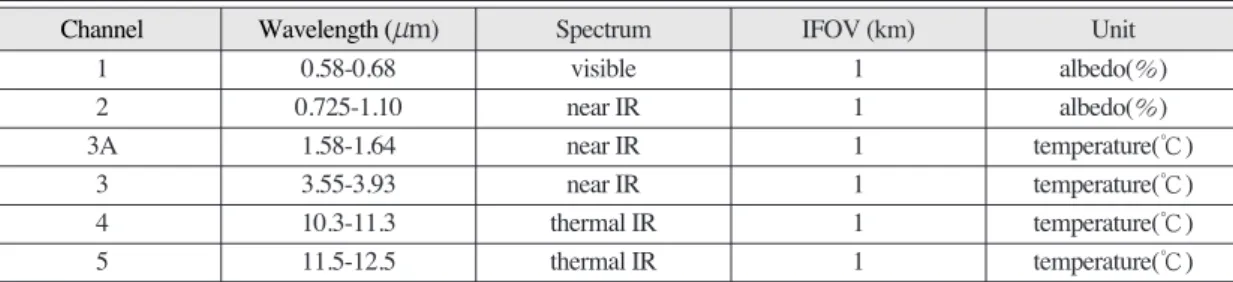
Table 1. Information of the NOAA/AVHRR channels
Channel Wavelength (mm) Spectrum IFOV (km) Unit
1 0.58-0.68 visible 1 albedo(%)
2 0.725-1.10 near IR 1 albedo(%)
3A 1.58-1.64 near IR 1 temperature(℃)
3 3.55-3.93 near IR 1 temperature(℃)
4 10.3-11.3 thermal IR 1 temperature(℃)
5 11.5-12.5 thermal IR 1 temperature(℃)
Channel Wavelength (mm) Spectrum IFOV (km) Unit
Fig. 1. Distribution of sea surface temperature (˚C) in the study area including the Yellow Sea, the East Sea, the Okhotsk Sea, and the Northwest Pacific.
2. Data
1) NOAA/AVHRR Data
We have obtained AVHRR data of NOAA-15, 17, 18, and 19 from Research Institute of Oceanography (RIO), Seoul National University (SNU) and National Meteorology Satellite Center (NMSC), Korea Meteorology Association (KMA). Table 1 presents the information of the AVHRR bands.
Instantaneous Field Of View (IFOV) of AVHRR is about 1 km at nadir. Both albedo data and brightness temperatures were used in the subsequent procedures of cloud removals and the estimation of SSTs (Table 1).
Since we were interested in the accuracy of satellite-observed SSTs for recent years, we selected NOAA data observed in 2009. For the previous NOAA satellites to NOAA-14, the accuracies of SSTs were already reported by Park et al.(1999). The year 2009 included all the NOAA satellites from NOAA- 15 to NOAA-19. The data in 2010 were excluded from the validation partly because the world-wide atmospheric and oceanic conditions in 2010 were beyond the past normal trend due to extreme La Nina event in 2010 (Hansen et al., 2010). A total 4,311 of NOAA passes were utilized in this study.
Due to unknown errors with the AVHRR instrument on NOAA-18, much of NOAA-18 data were missed from August to the end of 2009. NOAA- 19 was launched in February 2009 and started operating in July 2009, so that the AVHRR data for the first half in 2009 could not be available either.
However, we used all the NOAA-18 and NOAA-19 data because both the data could possibly reflect the seasonal characteristics.
2) Satellite-tracked Drifter Data
Many kinds of in-situ oceanic measurements can
be obtained from diverse equipments such as satellite-tracked drifters, moored buoys, CTD (Conductivity, Temperature, Depth), or other thermister measurements conducted at research vessels. In overall, water temperatures by ships and moored buoys correspond to bulk temperature and those were usually measured at different depths. It is necessary to obtain high quality in-situ measurements at similar water depths. In light of this, we selected only the drifters of which the temperature sensor kept almost the same depth (~20 cm) from the sea surface.
The satellite-tracked drifter data were obtained from Global Telecommunication System (GTS) data operationally used at KMA. For the most part, the precision of the drifter temperature is estimated to be fairly good for the validation of satellite-observed temperature. We collected the vast GTS drifters amounting to 713,179 in 2009 and sampled the data for the present study area as shown in Fig. 2, of which the colors denote the months of drifter measurements.
Most of the drifters were concentrated on the Kuroshio region in the Northwest Pacific. One of the most important advantage of the GTS drifter data is that the data can be measured simultaneously with the observations by NOAA satellites.
Fig. 2. Tracks of GTS drifters in the seas around Korea in 2009, where the colors denote the months of the drifters.
3. Method
1) Collocation Procedure
We have generated a matchup database between AVHRR data and drifter data as in-situ observations.
The overall flowchart of collocation procedure was presented in Fig. 3. First of all, all data of AVHRR were extracted from HRPT data and converted to albedos and brightness temperatures by the methods of the NOAA KLM User’s Guide(2007). For more accurate geometric registration, subjective navigation were then performed, which required lots of time.
In the production of the matchups, we collocated the two data sets within a spatial gap of about 1 km and a temporal interval of 30 minutes. The matchup database was composed of major data such as albedos and brightness temperatures, and other auxiliary information associated with the drifter data, including wind data if any. Additionally, satellite zenith angle and solar reflection angle were calculated for the collocation points. Statistics of each channel data such as maximum differences and
standard deviations within 3 by 3 window were archived in the database as well.
2) Removal of Pixels with Poor Angle Geometry
There are four angles related to geometry between a satellite and the sun such as a satellite zenith angle, solar zenith angle, solar reflection angle, and scattering phase angle. In order to eliminate a poor quality of SST induced by the poor geometry of satellite observation, we used the satellite zenith angle and the solar reflection angle. If the satellite zenith angle becomes large, the atmospheric path of radiances from the sea surface becomes elongated. If the solar reflection angle becomes small, the radiance reflected on the sea surface gives a sun glint on satellite. Thus, pixels with satellite zenith angle over 60˚ or solar reflection angle under 15˚ were excluded from the following steps to reduce errors (Bernstein, 1982).
3) Removal of Cloud Pixels
Since all the types of clouds are colder and more reflective than the ocean surface, the removal procedure of cloudy or cloud-contaminated pixels has been developed by giving thresholds on the reflectance and IR brightness temperatures. A series of uniformity tests were performed for the matchup data.
For daytime data, gross clouds were checked with albedos of AVHRR channel 2 and brightness temperatures of AVHRR channel 4 and 5. The pixel with albedo exceeding 3% or below -3.5˚C of the channel 4 or 5 bright temperatures was regarded as a cloud pixel and was excluded from the following procedure. The spatial uniformity was then tested with statistics, such as spatial mean, standard deviation, and difference between a maximum and a minimum of the albedos and brightness temperatures, within 3 by 3 window based on Sounders and Kriebel(1988). The final test was applied to semi- Fig. 3. The flowchart for the generation of matchup database
between NOAA/AVHRR data and satellite-tracked drifter data.
transparent cirrus clouds based on the method suggested by Závody et al.(2000).
In case of nighttime data, most of the procedures were the same with the daytime case except for the procedure of the albedo data. The daytime thresholds were empirically determined as described in the previous researches (Saunders and Kriebel, 1988;
Park et al., 1994).
4) Estimation of SST
We selected two representative algorithms, MCSST and NLSST, developed by NOAA/NESDIS (McClain et al., 1985; Walton, 1988; Walton et al., 1998) and used their coefficients to assess the accuracy of SSTs in the study region. The MCSST algorithm has a fundamental equation as the following form:
MCSST = AT11+ B(T11_ T12) + C(T11_ T12) (secq _ 1) + D(secq _ 1) + E, (1) where q is a satellite zenith angle and T11, T12are brightness temperatures for channel 4, 5 of AVHRR,
respectively. Walton et al.(1998) improved the MCSST algorithm by considering nonlinearity of SST depending on atmospheric moist condition as a function of water temperature and suggested the following form:
NLSST = AT11+ BTsfc(T11_ T12) + C(T11_ T12) (secq _ 1) + D(secq _ 1) + E, (2) where Tsfcis the first-guess SST. In this study, we used MCSST as a priori Tsfc. Table 2 presents the coefficients of split-window MCSST and split- window NLSST for daytime and nighttime satellite passes used in this study.
4. Results
1) Matchup Database
After the removal procedures of bad pixels with clouds or poor angles, a total of 1,070 matchups were remained in the matchup database (Table 3). Table 3 Table 2. The coefficients for sea surface temperature retrievals using MCSST and NLSST formula for NOAA satellites from NOAA-15, 17, 18, and 19
Satellite Method Time SST Retrieval Coefficients
A B C D E(C)
MCSST Day 0.959456 2.663579 0.570613 0.000 1.045
NOAA-15 Night 0.993892 2.752346 0.662999 0.000 0.084
NLSST Day 0.953493 0.087762 0.740922 0.0 1.64460
Night 0.890887 0.088730 0.557058 0.0 3.10170
MCSST Day 0.992818 2.49916 0.915103 0.000 -0.0177633
NOAA-17 Night 1.01015 2.58150 1.00054 0.000 -0.6675275
NLSST Day 0.936047 0.0838670 0.920848 0.000000 1.730238
Night 0.938875 0.0864265 0.979108 0.000000 1.430706
MCSST Day 1.02453 2.10044 0.784059 0.00000 -0.579631
NOAA-18 Night 1.00841 2.23459 0.736946 0.00000 -0.627809
NLSST Day 0.934004 0.0724457 0.748044 0.00000 1.815193
Night 0.939146 0.0750661 0.728430 0.00000 1.464730
MCSST Day 1.03851 1.72867 0.85261 0.00000 -0.7189935
NOAA-19 Night 1.00903 2.02274 0.68015 0.00000 -0.7184555
NLSST Day 0.94689 0.06355 0.80013 0.00000 1.5000035
Night 0.945190 0.065590 0.744790 0.00000 1.354560
Satellite Method Time SST Retrieval Coefficients
A B C D E(C)
shows the monthly distributions of the number of the matchups in 2009. The number of the matchups was significantly small in winter due to typical distributions of clouds generated by severe air-sea temperature differences. NOAA-19 was launched in February 2009 and started operating in July 2009, so there was no matchup point for NOAA-19 over the first half of 2009. The matchups of NOAA-19 might not represent the characteristic seasonal variations of SSTs because of the short period from June to December. In case of NOAA-18, the matchup pairs were pretty small especially for a couple of months from September to November. Except for the two cases of NOAA-18 and NOAA-19, other satellites continuously made observations over the entire year enough for the accuracy assessment of SST.
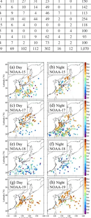
Fig. 4 shows the distributions of the matchups for day and night overpasses of NOAA satellites. Most of the matchups were concentrated in the Northwest Pacific and the East China Sea. Many matchups were found in the East Sea, however, they were limited only in the southern and southeastern regions. There were only a few points in the Yellow Sea and the Okhotsk Sea. For more accurate assessment of SSTs, it is important that the matchups should be uniformly distributed over the entire region both in terms of space as well as time. As shown in Fig. 4 and Fig. 5a, the months of the collocation data tended to be
concentrated in spring and autumn. In the East Sea, although there were many matchups, they were Fig. 4. Distributions of matchup points between NOAA/
AVHRR data and GTS drifter data in 2009, where the colors represent the months of the matchup points.
Table 3. Monthly distributions of the number of matchup points between NOAA/AVHRR data and GTS drifter data in 2009, where the symbol ‘_’represents no observations of NOAA19 during the pre-launch period from January to May in 2009
Satellite Time Jan Feb Mar Apr May Jun Jul Aug Sep Oct Nov Dec Total
NOAA-15 Day 3 3 6 5 26 14 11 27 31 23 1 0 150
Night 2 1 2 29 23 5 6 10 14 49 0 1 142
NOAA-17 Day 2 2 12 9 10 4 9 7 4 46 7 1 113
Night 3 10 20 10 36 21 18 41 44 49 2 0 254
NOAA-18 Day 7 10 15 31 28 15 6 4 0 0 0 2 118
Night 2 14 15 37 15 5 8 0 0 0 0 4 100
NOAA-19 Day - - - 1 4 11 9 62 4 2 93
Night - - - 4 7 2 10 73 2 2 100
Total 19 40 70 121 138 69 69 102 112 302 16 12 1,070
Satellite Time Jan Feb Mar Apr May Jun Jul Aug Sep Oct Nov Dec Total
mainly concentrated in southern part than in northern part from September to October as shown in Fig. 4a- 4d and Fig. 4h.
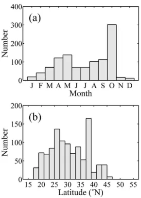
The histogram of the monthly distribution of matchup points in Fig. 5a revealed that the maximum frequency of the matchup numbers was found in October and the minimum from November to January next year. The latitudinal distributions of the matchups were abundant at mid-latitude regions, especially around 25˚N and 38˚N (Fig. 5b). By contrast, none of matchups was detected at high- latitude regions because of a few drifters.
2) Accuracies of SSTs
By using the brightness temperatures and NESDIS coefficients, the accuracies of MCSSTs and NLSSTs were estimated. Fig. 6a and 6b shows the comparisons between the satellite-observed SSTs and the drifter temperatures for the all matchups. Both MCSSTs and NLSSTs were well correlated with the drifter temperatures with correlation values of 0.9877 and Fig. 5. (a) Monthly and (b) latitudinal distributions of matchup
points between NOAA/AVHRR data and GTS drifter data in 2009.
Fig. 6. Comparisons of (a) MCSSTs and (b) NLSSTs with satellite SSTs and SST errors (satellite SST - buoy SST) for (c) MCSST and (d) NLSST algorithms.
0.9875, respectively. The accuracies of SSTs based on MCSST and NLSST algorithms seemed to be
quite similar with rms errors of 0.9590˚C and 0.9454˚C, respectively. NLSSTs tended to be slightly underestimated (bias of -0.0512˚C) and MCSSTs tended to be overestimated with a bias error of 0.0794˚C (Fig. 6c, 6d). Most of the collocation points were concentrated at a relatively high temperature range from 15˚C to 32˚C. By contrast, there were only a few SSTs near 3˚C. This indicates that more in-situ observations should be uniformly made even at low temperature ranges from -3˚C to -1.5˚C to enhance the accuracy of satellite SSTs. Since the study region included the Okhotsk Sea and the Russian coast in the East Sea with extremely low temperatures below 0˚C in winter, it would be more important to deploy the drifters in the seas.
Fig. 7 presents the comparisons between MCSSTs and drifter temperatures for day and night satellite overpasses. All the plots in Fig. 7 revealed that the two temperatures seem to be well correlated by showing linear relationship. In general, SST errors derived by near-polar orbit satellites were known to be less than 1 K approximately (McClain et al., 1985;
Walton, 1988; Vazquez et al., 1994; Walton et al., 1998). However, the individual points of the matchup database indicated that many of individual SSTs from satellite observations were deviated from oceanic in- situ measurements by greater than 1˚C. Especially, nighttime satellite-observed SSTs tended to be Fig. 7. Comparison of GTS drifter temperatures with sea
surface temperatures by the operational split window equations of NOAA/NESDIS for NOAA-15, 17, 18, and 19.
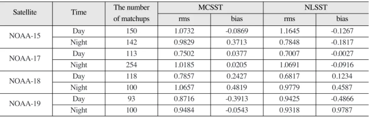
Table 4. SST errors (rms, bias) between sea surface temperature (MCSST, NLSST) from NOAA/AVHRR data and GTS drifter temperature for the satellites from NOAA-15, 17, 18, and 19
Satellite Time The number MCSST NLSST
of matchups RMS Bias RMS Bias
NOAA-15 Day 150 1.0732 -0.0869 1.1645 -0.1267
Night 142 0.9829 0.3713 0.7848 -0.1817
NOAA-17 Day 113 0.7502 0.0377 0.7007 -0.0027
Night 254 1.0185 0.0205 1.0691 -0.0916
NOAA-18 Day 118 0.7857 0.2427 0.6817 0.1234
Night 100 1.0657 0.4819 0.9779 0.4587
NOAA-19 Day 93 0.8716 -0.3913 0.9425 -0.4866
Night 100 0.9484 -0.0543 0.9318 0.9787
Satellite Time The number MCSST NLSST
of matchups rms bias rms bias
underestimated from drifter temperatures (Fig. 7).
SST errors (rms, bias) for each satellite and algorithm were listed in Table 4. Most of rms errors for day passes were smaller than night passes. This may be partly related to difficulty to eliminate cloud- contaminated pixels because of unavailability of visible channel data at night. NLSST algorithm was evaluated to be slightly more accurate than MCSST algorithm as presumed from the rms errors in Table 4, but no significant improvement unlike the previous literature (e.g., Walton et al., 1998). Although NOAA-19 matchups could not include the first half of 2009, the errors satisfied the reasonable limit of less than 1˚C. Daytime NOAA-18 NLSSTs showed the smallest rms error by 0.6817˚C followed by NOAA-17 MCSSTs 0.7502˚C. In overall, the rms errors were of less than 1℃ as similar to the previous literature for global ocean or local seas.
3) Characteristics of SST Errors
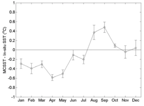
Fig. 8 is a plot of SST errors, differences between MCSSTs and drifter temperatures, as a function of time. The errors, averaged over each month, showed relatively low values within ±0.6˚C. However, the errors revealed seasonality in the way that the errors tended to be underestimated in winter and spring and overestimated by 0.4˚C in summer, particularly in August and September. This trend was coincident with the previous research of Park et al.(1994) performed in the East Sea.
The satellite SSTs have been reported to have dependency on the moisture amount in the atmosphere (e.g., Walton, 1988; Park et al., 1994;
Park et al., 1999). Fig. 9 also revealed the effect of atmospheric moist on SST errors as the previous literature. The amount of moist may be indirectly presumed from the difference between 11 mm and 12 mm brightness temperatures. The errors seemed to be underestimated at a range of somewhat dry condition
with brightness temperature differences (T11mm- T12mm) of less than 1.5˚C. Whereas, it tended to be overestimated at moist range from 1.5˚C to 3˚C of the brightness temperature differences. The temperature difference range with the most negative error was coincident with the driest condition near T11mm- T12mm values of less than 0.2˚C as shown in the scatter plots of the errors and binned error bars in Fig.
9. The reason for the dependence may be explained with the fact that moist air generally occurs over warm seas, so that atmospheric humidity increases with SST. Thus, MCSST errors were liable to be Fig. 8. Monthly variations of SST errors (MCSST - in-situ SST), where the bars represent the mean error of SST errors (s / n-1) for each month.
Fig. 9. Distributions of SST errors (MCSST - in-situ SST) as a function of brightness temperature differences (T11mm-T12mm), where the bars represent the standard deviation of SST errors (s) for each interval.
overestimated at high temperature ranges in the low- latitude subtropical oceans. In light of this, it may be quite difficult to satisfy both atmospheric conditions if the study region is so wide as to have extremely dry and moist conditions.
Under very humid condition, the satellite observed brightness at infrared window channels tends to be attenuated by intervening atmospheric water vapour.
The dependence of the SST errors on atmospheric moist conditions in the study region implied that the NESDIS equations could not be completely applicable for all regions in spite that the equation itself already included the effect of the attenuation by water vapour.
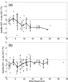
Some drifters, called Surface Velocity Program (SVP), can carry sensors that measure temperature, salinity, wind direction, ambient sound to calculate wind speed and rain rate. Out of the 1,070 matchups, 202 points have wind speed measurements with 70 daytime points and 132 nighttime points. We analyzed the effect of wind speed on SST errors. Fig.
10 shows the distributions of daytime and nighttime SST errors (MCSST - in-situ SST) as a function of wind speed (m/s), where the bars represent the standard deviation (s) of SST errors for each interval.
For daytime passes, the errors seemed to be decreased as wind blew increasingly. By contrast, those errors tended to be slightly increased as wind speeds increased. Donlon et al.(1999) characterized the wind dependence in the comparison between satellite SST and shipboard bulk SST measurements. The most positive wind effects on SST were found when wind speeds occurred at the low range of less than 5 m/s (Fig. 10a). In nighttime, the wind forcing was likely to become less important when wind blew strongly.
SST changes seemed to be less sensitive to wind effects for high winds of greater than 15 m/s, whereas they were more or less underestimated at low winds of less than 7 m/s (Fig. 10b).
The dependence of SST errors on wind speeds, particularly at low wind speeds, primarily originated from the skin-bulk differences due to changes in the vertical stability of water column. Details about regional dependence on differences between drifter measurements and CTD temperature measurements were depicted in the previous literature (e.g., Donlon et al., 1999; Park et al., 2008).
5. Summary and Conclusion
In this study, we produced a total 1,070 matches of co-located and co-temporal NOAA satellites (NOAA-15, 17, 18, and 19) and drifter data in 2009.
The error estimates of all satellite-derived MCSSTs and NLSSTs by NESDIS coefficients indicated that satellite-observed SSTs showed a reasonable agreement with drifter temperatures on average.
Fig. 10. Distributions of (a) daytime and (b) nighttime SST errors (MCSST - in-situ SST) as a function of wind speed (m/s), where the bars represent the standard deviation of SST errors (s) for each interval.
Although significant missings in the matchup database were found for NOAA-18 and NOAA-19 satellites for several months, rms and bias errors for both MCSSTs and NLSSTs, in most of the cases, showed a reasonable rms errors of about 1.0˚C (0.75- 1.16˚C). NLSST algorithm presented errors similar to MCSST algorithm without any significant improvement in the study region, which was contrast with the previous researches concerning its improved accuracy (Walton, 1988; Walton et al., 1998).
In addition, this study presented that satellite- observed SSTs have been affected by oceanic and atmospheric conditions. The SST errors revealed various dependences on latitude, seasonal variations, and wind speed. On average, satellite MCSSTs tended to be underestimated by -0.6˚C in maximum in winter and spring, whereas overestimated by 0.4˚C in summer. The significant dependence on dry or moist atmospheric condition implies that NESDIS coefficients should be optimized to the regional seas by deriving new coefficients in the SST equations.
Wind forcings also presented their influences on SST errors, particularly at low wind speeds of less than 5 m/s. Since there were not too many wind observations by drifters in this study, the tendency of SSTs on wind speeds might not be robust. However, in spite of the small number of the wind measurements, the general trend were coincident with the previous research (Donlon et al., 1999) on the different response of the skin-bulk SST differences to wind forcings.
During El Niño and La Niña years, SSTs in the northeast Asian seas were reported to be much deviated from SSTs in summer and winter than those in the normal years (Wang et al., 2000; Wang and Zhang, 2002). Since a severe El Niño event occurred during the study period, for more details, a better and more matchups between satellite and in-situ measurements should be collected by extending the
matchup database for a longer period.
SST is one of the most important oceanic and atmospheric parameters for diverse applications such as understanding of oceanic processes, air-sea interactions, fisheries, weather forecast, and so on. In light of this, it should be continuously validated to keep a required accuracy for the diverse applications.
The characteristics of SST errors should be also investigated and understood. Without deep understanding on the errors, applications of SSTs should be limited as evident from the amplification of erroneous SSTs in the numerical models and data assimilation procedure.
NOAA satellites will be successively launched in the future. Although NESDIS will produce SST coefficients continuously, efforts for regional validation should be consecutively made by conducting cruise campaigns for in-situ temperature measurements and persistent deployment of drifters.
This study addressed the necessity of the SST equations optimized to the local seas around Korea from the viewpoint of regional purposes.
Acknowledgement
This study was supported by KMA (Korea Meteorology Association) / NMSC (National Meteorology Satellite Center). NOAA satellite data from SNU/RIO were supported by EAST-1 project of MLTC (Ministry of Land, Transport and Maritime Affairs). We are also very grateful to two unknown reviewers for their helpful comments.
References
Bernstein, R. L., 1982. Sea surface temperature estimation using the NOAA-6 Satellite
Advanced Very High Resolution Radiometer, Journal of Geophysical Research, 87(C12):
9455-9465.
Donlon, C. J., T. J. Nightingale, T. Sheasby, J.
Turner, I. S. Robinson, and W. J. Emergy, 1999. Implications of the oceanic thermal skin temperature deviation at high wind speed, Geophysical Research Letters, 26(16):
2505-2508.
Hansen, J., R. Ruedy, M. Sato, and K. Lo, 2010.
Global surface temperature change, Reviews of Geophysics, 48: RG4004.
Kilpartrick, K. A., G. P. Podesta, and R. Evans, 2001.
Overview of the NOAA/NASA advanced very high resolution radiometer Pathfinder algorithm for sea surface temperature and associated matchup database, Journal of Geophysical Research, 106(C5): 9179-9197.
Lee, M. A., Y. Chang, F. Sakaida, H. Kawamura, C.
H. Cheng, J. W. Chan, and I. Huang, 2005.
Validation of Satellite-Derived Sea Surface Temperatures for Waters around Taiwan, Terrestrial, Atmospheric and Oceanic sciences, 16(5): 1189-1204.
McClain, E. P., W. G. Pichel, and C. C. Walton, 1985. Comparative performance of AVHRR- based Multichannel sea surface temperatures, Journal of Geophysical Research, 90(C6):
11609-11618.
McClain, E. P., 1989. Global sea surface temperatures and cloud clearing for aerosol optical depth estimates, International Journal of Remote Sensing, 10(4-5): 763-769.
McMillin, L. M. and D. S. Crosby, 1984. Theory and Validation of the Multiple Window Sea Surface Temperature Technique, Journal of Geophysical Research, 89(C3): 3655-3661.
Goodrum, G., K. B. Kidwell, and W. Winston, 2007.
NOAA KLM user’s guide, Technical Report,
National Environmental Satellite, Data, and Information Services (NESDIS).
Park, K. A., J. Y. Chung, K. Kim, and B. H. Choi, 1994. A study on comparison of satellite drifter temperature with satellite derived sea surface temperature of NOAA/NESDIS, Korean Journal of Remote Sensing, 11(2):
83-107.
Park, K. A., J. Y. Chung, K. Kim, B. H. Choi, and D.
K. Lee, 1999. Sea Surface Temperature Retrievals Optimized to the East Sea (Sea of Japan) using NOAA/AVHRR Data, Marine Technology Society Journal, 33(1): 23-35.
Park, K. A., J. Y. Chung, K. Kim, and P. C.
Cornillon, 2005. Wind and bathymetric forcing of the annual sea surface temperature signal in the East (Japan) Sea, Geophysical Research Letters, 32: L05610.
Park, K. A., F. Sakaida, and H. Kawamura, 2008.
Oceanic Skin-Bulk Temperature Difference through the Comarison of Satellite-Observed Sea Surface Temperature and In-Site Measurements, Korean Journal of Remote Sensing, 24(4): 273-287.
Prabhakara, C., G. Dalu, and V. G. Kunda, 1974.
Estimation of Sea Surface Temperature from Remote Sensing in the 11 mm to 13 mm Window, Journal of Geophysical Research, 79(33): 5039-5044.
Sakaida, F. and H. Kawamura, 1992. Estimation of sea surface temperatures around Japan using the advanced very high resolution radiometer, (AVHRR)/NOAA-11, Journal of Oceanography, 48(2): 179-192.
Saunders, R. W. and K. T. Kriebel, 1988. An improved method for detecting clear sky and cloudy radiances from AVHRR data, International Journal of Remote Sensing, 9(1): 123-150.
Strong, A. and E. P. McClain, 1984. Improved ocean surface temperatures from space_Comparisons with drifting buoys, Bulletin of the American Meteorological Society, 65(2): 138-139.
Vazquez, J., A V. Tran, R. Sumagaysay, E. Smith, S.
Digby, and K. Perry, 1994. NOAA/NASA AVHRR Oceans Pathfinder Sea Surface Temperature Data Set User’s Handbook.
Walton, C. C., 1988. Nonlinear multichannel algorithms for estimating sea surface temperature with AVHRR satellite data, Journal of Applied Meteorology, 27: 115-124.
Walton, C. C., W. G. Pichel, J. F. Sapper, and D. A.
May, 1998. The development and operational application of nonlinear algorithms for the measurement of sea surface temperatures with the NOAA polar-orbiting environmental satellites, Journal of Geophysical Research, 103(C12): 27999-28012.
Wang, B., R. Wu, and X. Fu, 2000. Pacific-East Asian Teleconnection: How Does ENSO Affect East Asian Climate?, Journal of Climate, 13: 1517-1536.
Wang, B. and Q. Zhang, 2002. Pacific-East Asian Teleconnection. Part II: How the Philippine Sea Anomalous Anticyclone is Established during El Nino Development, Journal of Climate, 15: 3252-3265.
Yashayaev, I. M. and I. I. Zveryaev, 2001. Climate of the seasonal cycle in the North Pacific and the North Atlantic oceans, International Journal of Climatology, 21(4): 401-417.
Závody, A. M., C. T. Mutlow, and D. T. Llewellyn- Jones, 2000. Cloud Clearing over the Ocean in the Processing of Data from the Along- Track Scanning Radiometer (ATSR), Journal of Atmospheric and Oceanic Technology, 17:
595-615.