Accuracy and Error Characteristics of SMOS Sea Surface Salinity in the Seas around Korea

(1)

J. Korean Earth Sci. Soc., v. 41, no. 4, p. 356

−

366, August 2020 https://doi.org/10.5467/JKESS.2020.41.4.356

ISSN 1225-6692 (printed edition) ISSN 2287-4518 (electronic edition)

Accuracy and Error Characteristics of SMOS Sea Surface Salinity in the Seas around Korea

Kyung-Ae Park

^1,2,

* and Jae-Jin Park

³

1

Department of Earth Science Education, Seoul National University, Seoul 08826, Korea

2

Research Institute of Oceanography, Seoul National University, Seoul 08826, Korea

3

Department of Science Education, Seoul National University, Seoul 08826, Korea

Abstract: The accuracy of satellite-observed sea surface salinity (SSS) was evaluated in comparison with in-situ salinity measurements from ARGO floats and buoys in the seas around the Korean Peninsula, the northwest Pacific, and the global ocean. Differences in satellite SSS and in-situ measurements (SSS errors) indicated characteristic dependences on geolocation, sea surface temperature (SST), and other oceanic and atmospheric conditions. Overall, the root-mean-square (rms) errors of non-averaged SMOS SSSs ranged from approximately 0.8-1.08 psu for each in-situ salinity dataset consisting of ARGO measurements and non-ARGO data from CTD and buoy measurements in both local seas and the ocean. All SMOS SSSs exhibited characteristic negative bias errors at a range of −0.50- −0.10 psu in the global ocean and the northwest Pacific, respectively. Both rms and bias errors increased to 1.07 psu and −0.17 psu, respectively, in the East Sea. An analysis of the SSS errors indicated dependence on the latitude, SST, and wind speed. The differences of SMOS-derived SSSs from in-situ salinity data tended to be amplified at high latitudes (40-60^oN) and high sea water salinity. Wind speeds contributed to the underestimation of SMOS salinity with negative bias compared with in-situ salinity measurements. Continuous and extensive validation of satellite-observed salinity in the local seas around Korea should be further investigated for proper use.

Keywords: SMOS, Sea surface salinity, ARGO, East Sea, satellite salinity error

Introduction

Sea surface salinity (SSS) is one of the most important oceanic variables to affect the ocean circulation and global hydrological cycle. It has been played key roles in controlling and regulating recent climate change, water exchange between ocean and atmosphere, and diverse oceanic processes (Curry et al., 2003; Lagerloef et al., 2008; Klemas, 2011).

It has long been impossible to observe the spatial distribution of sea surface salinity from in-situ salinity measurements until the SMOS (Soil Moisture and Ocean Salinity) of the European Space Agency’s (ESA) launched on 2 November 2009. It is passive L-

band interferometric radiometer at a frequency of about 1.4 GHz. Aquarius/SAC-D satellites, with an active L-band radar scatterometer integrated with the passive L-band radiometer, have been successfully launched on June 2011 (Lagerloef et al., 1995;

Bingham et al., 2002). Soil Moisture Active Passive (SMAP), launched on 31 January 2015, is the latest satellite to observe SSS as one of NASA environmental monitoring satellites. These satellites have contributed to understand terrestrial water, energy balance, and carbon cycles, to estimate global water fluxes, and to enhance weather and climate forecast skill. The three satellites have contributed to produce the distribution of SSS can have been observing over a wide area of the ocean in near real-time (Font et al., 2004; LeVine et al., 2007; Tranchant et al., 2008).

The SMOS was the first satellite to observe SSS in the global ocean and long-lived over 10 years (completed on the10-th year in orbit in November 2019). It has continuously provided SSS data with the help of stable sensor with comparative quality. The

*Corresponding author: [email protected]

*Tel: +82-2-880-7780

This is an Open-Access article distributed under the terms of the Creative Commons Attribution Non-Commercial License (http://

creativecommons.org/licenses/by-nc/3.0) which permits unrestricted non-commercial use, distribution, and reproduction in any medium, provided the original work is properly cited.

(2)

SSS data has been used in hydrological, oceanographic and atmospheric models. The SSS data explored the impacts of salinity on air-sea heat fluxes and dynamics affecting large-scale processes of the Earth’s climate system.

Many of studies have already investigated the accuracy of SSS in the global ocean as well as in regional seas (Abe and Ebuchi, 2014; Bhaskar and Jayaram, 2015; Boutin et al., 2013; Drucker and Riser, 2014; Kim et al., 2014; Ratheesh et al., 2013; Tang et al., 2014). Its expected accuracy has known to be 0.2 psu for a monthly average within 1

^o

×1

^o

(Lagerloef and Font, 2010). Besides the overall average, satellite SSSs compared to in-situ measurements have shown rms errors less than 0.5 psu such as were done to 0.42 psu (Abe and Ebuchi, 2014; Drunker and Riser, 2014), 0.31 psu (Reagan et al., 2014), 0.495 psu (Tang et al., 2014), or 0.45 psu (Ratheesh et al., 2013) in the global ocean. Somewhat larger SSS errors were found in the regions such as high-latitude regions, Atlantic Ocean near the Amazon River with considerable river input, intertropical convergence zone, especially Eastern Pacific Fresh Pool, and South Pacific Convergence Zone (SPCZ) (Tang et al., 2014). Some of studies referred potential error sources as the difference of measurement depths between a satellite within 2-3 cm from the sea surface and a top measurement of ARGO (Array for Real-time Geostrophic Oceanography) float at depths of 1-7 m (Drucker and Riser, 2014). The differences induced errors greater than −0.1 psu when precipitation gave a rise to a change in vertical stability of the upper surface layer (Drucker and Riser, 2014).

It is important to understand how accurate the SMOS SSS in the local seas around Korean peninsula including the East Sea and in the northwest Pacific.

The SSS errors in the local seas should be compared with the accuracy of SSS in global ocean. Therefore, the objectives of this study are (1) to assess the accuracy of satellite SSS as compared with in-situ salinity measurements in the northwest Pacific Ocean and the East Sea, (2) to compare with the SSS accuracy in the global ocean, (3) to examine the

characteristics and dependences of SSS errors on atmospheric and oceanic parameters.

Data

Satellite data

To validate the accuracy of satellite-observed SSS and understand the characteristics of the errors, we used level-2 SMOS data of ESA from January 2010 to December 2013. Quality flags of SSS measurements were also used to eliminate abnormal pixels associated with sea ice, land, heavy rainfall, other contaminations for the best data for the estimation of the accuracy.

Fig. 1a illustrates an example of SMOS SSS map averaged for the period of 2012 to 2013, which obviously presents distinctive salinity between the Atlantic Ocean with relatively high salinity (>36 psu) and the Pacific Ocean (33-36 psu). Fig. 1b presents the spatial distribution of SMOS SSS observations on 30 April 2013 in the global ocean.

In-situ salinity measurements

Satellite SSS data are compared with surface salinity data from ARGO floats at the depth nearest the sea surface. ARGO data from ARGO data Center and Global Data Assembly Centres (GDAC) (ftp://ftp.

ifremer.fr/ifremer/argo) were used. To do so, quality- controlled ARGO data, passing through real-time and delayed mode processing, were used to evaluate the accuracy of satellite salinity. The salinity data of World Ocean Database (WOD) 2013 (WOD13) were also obtained from the National Oceanographic Data Center (NODC) (Conkright et al., 2002). The database includes moored buoy data, ship-of-opportunity CTD casting data, and glider data.

Methods

Matchup procedure

Prior to the production of the matchup database

between satellite SSS and in-situ measurements,

SMOS SSS data with poor quality were eliminated

through a few of steps. First of all, pixels of very low

(3)

358

Kyung-Ae Park and Jae-Jin Park

SST below 5

^o

C were discarded since sensitivity of a satellite sensor at L-band frequency was very low not enough to retrieve SSS adequately from emitted surface radiance (Abe and Ebuchi, 2014; Yueh et al., 2001).

A collocation database between the satellite salinity data and the in-situ observations was produced by giving a spatial gap of about 100 km and a temporal interval of 12 hours. The matchup database was composed of satellite salinity, in-situ salinity, time, geolocation information, depths of in-situ salinity, as well as other auxiliary information such as wind speed and SST.

Results

Distribution of matchup points

To understand the gross errors and uncertainties of

SMOS SSS in the seas around Korea, we made a

matchup database between satellite data and in-situ

salinity measurements. Since ARGO salinity data prior

to a series of quality control processes have known to

be biased with time (Wong et al., 2003), we performed

the evaluation of accuracies for the classified cases of

the salinity data from all instruments, including or

excluding the ARGO data, and other salinity data

except for ARGO data as shown in Table 1. To

examine SSS errors quantitatively under common

conditions, satellite SSSs observed under poor

conditions such as low SST (<5

^o

C) and high winds

(>15 m s

⁻¹

) were eliminated (e.g., Abe and Ebuchi,

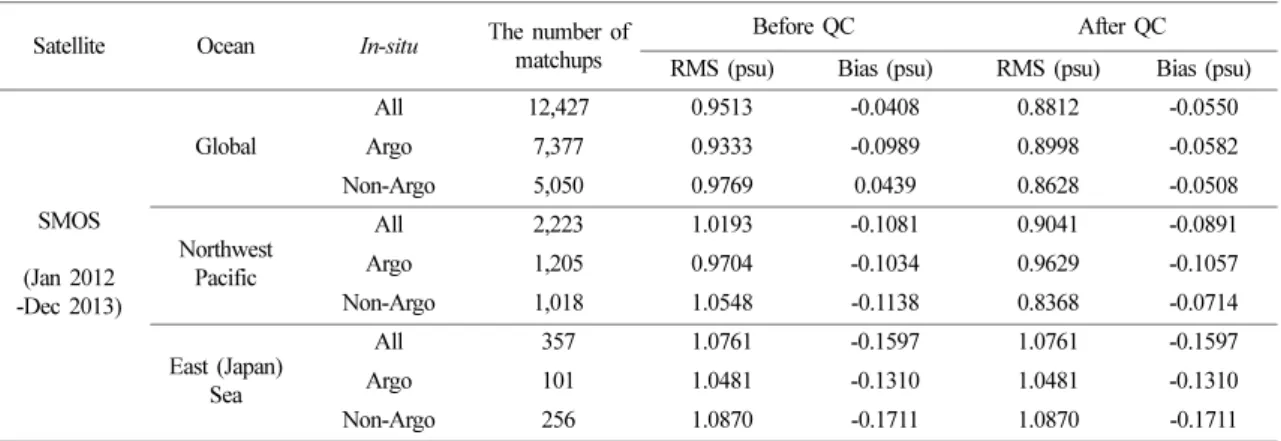
2014) prior to the estimation of the errors. Table 1

expresses the numbers of the collocated data pairs and

errors of satellite SSS before and after the quality

control (QC) processes. The numbers of collocation

points of the SMOS in the global ocean were 12,427

Fig. 1. (a) Spatial distribution of SMOS sea surface salinity (SSS) from SMOS in the global ocean and (b) SSS within the swath of satellite observation for a day 1 January 2013.

(4)

for the study periods from January 2012 to December 2013.

Figure 2 illustrates the spatial distributions of the collocated points between SMOS and in-situ salinity measurements including ARGO float data. The matchup points seem to cover most of the global ocean except for some regions near the Antarctic Ocean and some of marginal seas such as the Okhotsk Sea, the Yellow Sea, and the East China Sea. There are no matchups in the Yellow Sea because ARGO floats have not been deployed in the Yellow Sea due to the shallow bathymetry less than 100 m. The matchups are uniformly distributed over the entire region in terms

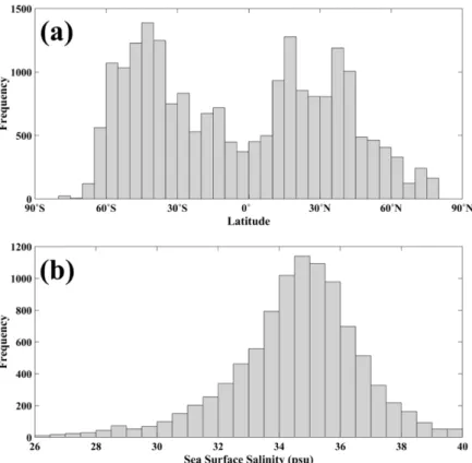
of both space and a range of SSSs from low salinity of about 26 psu to about 40.0 psu as shown in Fig.

3b. High number frequencies over 1000 were found at a range between 34 and 36 psu. The frequency of the salinity data was extremely low above the two ranges, especially lower than 28 psu or higher than 38 psu.

As illustrated in Fig. 3a, the latitudes of the collocated points were mostly distributed at mid- latitude regions around 40

^o

S, 25-35

^o

N. There is a lack of matchups in only a few collocations, particularly at high latitudes greater than 60

^o

N or 60

^o

S. This might be due to lack of ARGO floats near polar regions.

Table 1. RMS and bias errors of satellite-observed sea surface salinity in the global ocean, the northwest Pacific Ocean, and the East Sea for the datasets classified into all of in-situ measurements, ARGO float data, and non-ARGO data before and after quality control processes of the salinity data

Satellite Ocean In-situ The number of matchups

Before QC After QC

RMS (psu) Bias (psu) RMS (psu) Bias (psu)

SMOS (Jan 2012 -Dec 2013)

Global

All 12,427 0.9513 -0.0408 0.8812 -0.0550

Argo 7,377 0.9333 -0.0989 0.8998 -0.0582

Non-Argo 5,050 0.9769 0.0439 0.8628 -0.0508

Northwest Pacific

All 2,223 1.0193 -0.1081 0.9041 -0.0891

Argo 1,205 0.9704 -0.1034 0.9629 -0.1057

Non-Argo 1,018 1.0548 -0.1138 0.8368 -0.0714

East (Japan) Sea

All 357 1.0761 -0.1597 1.0761 -0.1597

Argo 101 1.0481 -0.1310 1.0481 -0.1310

Non-Argo 256 1.0870 -0.1711 1.0870 -0.1711

Fig. 2. Spatial distribution of the collocation points between SMOS sea surface salinity (SSS) and in-situ salinity measurements in the global ocean.

(5)

360 Accuracy of sea surface salinity in the global ocean

Prior to the assessment of the accuracy of the SMOS data in the local seas around Korea, the accuracy of the salinity in the global ocean was estimated. The matchup database was classified into two groups as ARGO data and non-ARGO data, and then classified again into two groups, with performing and not performing QC process.

Table 1 summarizes the performances of the SMOS salinity validation over the global ocean, the northwest Pacific, and the East Sea with the rms error, bias for all data, ARGO data only, non-ARGO data before and after applying QC procedure of the salinity data.

Overall, there were not specific differences of the rms errors between ARGO salinity data and non-ARGO data, which gave an evidence of high performance of the bias correction through real-time and delayed QC processes.

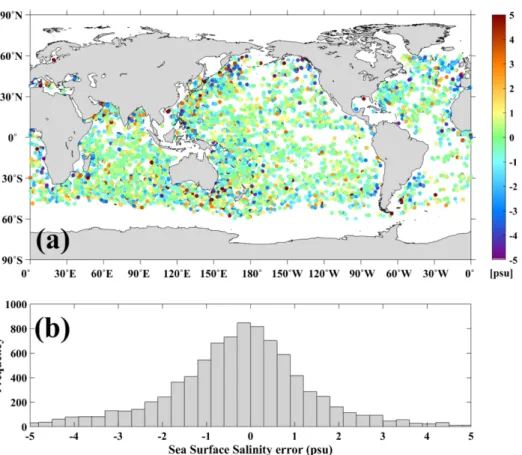
Figure 4 illustrates the spatial distributions of the SMOS salinity differences between SSS and in-situ salinity (satellite minus in-situ). The differences ranged from −5.0 to 5.0 psu globally. Rms error of SMOS SSS for all data in the global ocean was about 0.9513 psu (before QC) and 0.8812 psu (after QC), with bias errors of about −0.0408 and −0.0550 psu, respectively (Table 1). For the ARGO data, the rms error of 0.9333 psu (before QC) was slightly improved with relatively small rms error of about 0.8998 psu after the QC procedure of the ARGO salinity data. Other data without containing any ARGO data showed a similar accuracy with the rms error of 0.9769 psu (0.8628 psu) and a bias error of about 0.0439 psu (−0.0508 psu) in case of performing QC (non-QC) procedure (Table 1).

Figure 5 illustrates the comparisons of the SMOS

SSS values and in-situ salinity measurements. Apparently,

most of the SMOS SSSs showed weak agreement

Fig. 3. Histograms of the number of the matchup data between SMOS sea surface salinity (SSS) and in-situ salinity measurements in the global ocean with respect to (a) latitude and (b) SSS (psu).

(6)

with the drifter temperatures. When we focused on the small range of salinity from 34 to 36 psu, there are relatively good relationship by showing linear coincidence.

However, there are high scattering points with differences exceeding 4.0 psu at ranges with small number frequencies (log-scale) as denoted in colors in Fig. 5.

Accuracy of sea surface salinity in the northwest pacific

Figure 6 indicates the comparisons of the satellite SSSs with in-situ salinity measurements in the north- west Pacific Ocean, where the matchup points of the East Sea are omitted for the comparison in the next section. The scatter plot of the SSS differences in Fig.

6a shows relatively a large range of the salinity differences from −2.0 to 2.0 psu. The number of the

matchup points in the northwest Pacific amounted to 2,223 consisting of 1205 ARGO drifter observations and 1018 from CTD and other measurements (Table 1). The SMOS SSSs before quality control procedure of in-situ salinity data showed the rms error of 1.093 psu and bias of −0.1081 psu. In case of applying QC procedure, the rms and bias errors were slightly decreased to 0.9041 psu and −0.0891 psu, respectively (Table 1). The matchups of ARGO data only amounting to 1,205 indicated some improved accuracy of rms error of about 0.9704 psu and bias error of −0.1034 psu. Exclusion of the AGRO data from the matchup database revealed a slightly lower accuracy by showing the rms (1.0548) and bias errors ( −0.1138) before the QC procedure and 0.8368 and −0.0714 psu after the QC procedure, respectively (Table 1).

It seems that SMOS SSSs did not well coincided

Fig. 4. (a) Spatial distribution of SMOS sea surface salinity (SSS) differences from in-situ measurements (satellite minus in-situ) in the global ocean and (b) the histogram of the number of the SSS differences between SMOS SSS and in-situ salinity measurements in the global ocean.

(7)

362 with in-situ measurements as noted in the scatter plots for the northwest Pacific region (Fig. 6b). In-situ salinity shows a distribution at a relatively small range of salinity from 32 to 35.5 psu. Contrast to this, the SMOS SSS was estimated at a large range from 30 to 39 psu as shown in Fig. 6b. However, there exists a positive tendency that a majority of SSSs occupying the largest fraction are distributed on the linear line centered at about 34 psu.

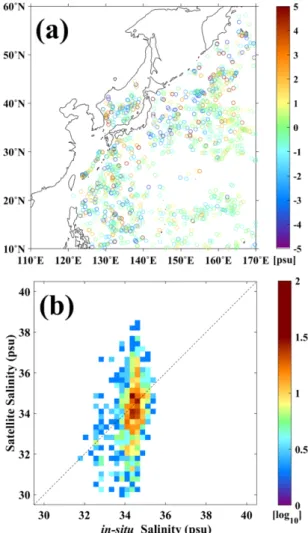
Accuracy of sea surface salinity in the east sea

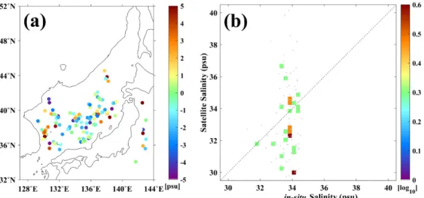
Figure 7a presents the scatter plot of the differences between the satellite SSSs and in-situ salinity (satellite minus in-situ) in the northwest Pacific for the study period. The salinity differences distributed at a range from −2.0 to 2.0 psu and presented no peculiar features in terms of their spatial distributions and the difference. The differences were irregularly distributed without any dependence on a distance from the coast or latitudinal dependence (Fig. 7a).

Figure 7b shows the 2-D histogram of the number density within a given bin of 0.2×0.2 psu of in-situ salinity and satellite SSS. Although the rms error (1.0761 psu) and bias (−0.1597 psu) of all SSSs in the

East Sea are comparatively similar to those of the northwest Pacific (Table 1), the comparison of SSS and in-situ salinity is considered to have failed to show good correlation. For instance, if the surface salinity is 34 psu, the SSS observed by the satellite can be varied significantly from 30 to 37 psu. The rms errors showed similar values, such as 1.0481, 1.0870, 1.0481, and 1.0870 psu, regardless of whether QC was executed or how data was observed such as CTD or ARGO float (Table 1). The bias errors of SSSs in the East Sea changed with a small difference within the range from −0.1310 to −0.1711. All of

Fig. 6. (a) Spatial distribution of SMOS surface salinity errors from in-situ measurements (satellite minus in-situ) in the northwest Pacific, and (b) their number density histograms on logarithmic scale.

Fig. 5. Comparison of SMOS data and in-situ salinity, where the colors represent the number density of each bin of salinity values on logarithmic scale.

(8)

these results implied that SMOS SSSs should be carefully checked their possibility for the purpose of the oceanic applications.

Discussion

In the previous section, satellite SSSs in the East

Fig. 7. (a) Spatial distribution of collocated SMOS surface salinity differences from in-situ measurements (satellite minus in-situ) in the East Sea, and (b) their number density histograms on logarithmic scale.

Fig. 8. SMOS sea surface salinity errors (psu) from in-situ measurements (satellite minus in-situ) in the global ocean with respect to (a) latitude, (b) sea surface temperature (^oC), (c) salinity, and (d) wind speed (m s⁻¹), where the error bar represents a mean error (σ /

N 1 –

), N the number of the matchup data points each interval.

(9)

364 Sea exhibited relatively poor rms errors, while those of the global ocean revealed relatively good coincidences.

It is meaningful to understand the conditions related to the satellite SSS errors. First, we investigated the characteristics of the SSS errors in terms of geolocation.

Other potential error sources were also discussed regarding the effects of sea surface temperature, sea water salinity, and wind speed.

Dependence on latitude

Figure 8a illustrates satellite SSS errors, the differences of the satellite SSS from the drifter temperatures, with respect to latitude in the global ocean. Although each individual SSS scattered over a wide range of the differences amounting to 2.0 psu as marked in Fig. 4a, the mean value of each bin showed relatively good errors. There is a peculiar tendency of the errors such as negative differences of less than 0.3 psu at low latitudes within 20

^o

N from the equator and the southern hemisphere. As goes to the high-latitude regions (20-60

^o

N), the errors tended to be amplified especially. This might be reduced by degraded measurement precision and could be improved by averaging with greater sampling frequency as a polar orbiting satellite (Lagerloef and Font, 2010).

Effect of sea surface temperature

Satellite salinity tends to be poorly estimated at low sea water temperatures because of less sensible response of a passive microwave SSS sensor at L-band frequency (Lagerloef and Font, 2010). The sensitivity becomes largest at the highest temperatures and yields better measurement precision in warm versus cold ocean conditions (Lagerloef and Font, 2010). Figure 8b indicates that the SSS errors indicated a somewhat different feature by negative values over the whole temperature range. the SSS errors of the global ocean were negatively correlated with SST with a slope of

−0.0216 psu

^o

C

⁻¹

(p=1.91×10

⁻⁹

, 95% confidence). The SSS errors were smallest at a temperature of about 15

^o

C. Effect of sea water salinity

Figure 8c shows the SMOS salinity differences from in-situ salinity with respect to surface salinity.

One of interesting feature is that the differences tended to increase at a range of high salinity. The SMOS salinity tends to be poorly estimated at high sea water salinity. The differences decreased to −2.5 psu when the sea water had a salinity of 38.5 psu.

The SMOS salinity showed small errors at a range of low salinity of less than 31 psu as shown in Fig. 8c.

This implies that the satellite SSS can be estimated with satisfaction when the sea water salinity is low in the fresh regions such as a zone of river discharge.

Effect of wind speed

Since the passive microwave sensor is mostly affected by surface roughness, the wind speeds affecting surface roughening perhaps have influences on the SSS errors (Yueh et al., 2013). This conjecture was investigated to examine the errors of the global ocean as a function of wind speed in Fig. 8d. The errors did not show any peculiar dependence at overall wind speeds from 1 m s

⁻¹

to 10 m s

⁻¹

. At a range of about 2 m s

⁻¹

, they were relatively small of about 0.2 psu.

At high wind speeds near 10 m s

⁻¹

, satellite SSSs tended to be smaller than in-situ salinity. The distributions on wind dependence have been demonstrated by the previous studies (e.g., Abe and Ebuchi, 2014).

This investigation implies that the surface salinity can be moderately changed the accuracy of the estimation of satellite SSS. Atmospheric conditions such as heavy rainfall and evaporations might have influences on the accuracy of the SSSs, especially with the dominant activities of sea surface wind field (Jacob and Koblinsky, 2007).

Other potential causes

In addition to the factors causing SMOS salinity data errors, as mentioned earlier, there are various errors related to ARGO, CTD, and moored buoy data.

Observational errors result from the instruments

(10)

themselves, and stability problems reduce accuracy in real-time and delayed-mode QC procedures for ARGO salinity data. Differences in observed depths by different instruments can lead to further issues. The observation depth of the ARGO float closest to the sea surface fluctuates around 3-10 m. The observation depths of the CTD and the buoy measurements are also different. Because the satellite salinity products have been verified with such in-situ measurements, it may not be accurate as to the depth of the satellite salinity. These problems will require more consistent and continuous in-depth research in the future.

Conclusion

In this study, we investigated the accuracies of SSS in the seas around Korea, northwest Pacific Ocean, and the global ocean for the period of 2012-2013 by comparison with in-situ salinity measurements from ARGO floats, moored buoys, many of ship-opportunity CTD measurements. As a result, SMOS SSS errors presented characteristic dependence on latitudes, but they were mostly underestimated at all ranges of SST, salinity, and wind speed.

However, a partial coincidence of satellite SSSs with ARGO SSSs does not necessarily signify that satellite salinity can be directly used in all researches over the whole regions of the ocean. It still has many of limitations at high latitude regions greater than 40

^o

N with very low water temperatures. Thus, satellite SSS should be cautiously used for further applications.

Nevertheless, the accuracy and error characteristics of SSS disclosed herein are believed to enhance our understanding of one of potential sources of SSS variations. In-depth studies on the accuracy of Aquarius and SMAP SSSs should be performed in the seas around Korea in the near future.

Acknowledgments

This work was supported by the National Research Foundation of Korea (NRF), grant funded by the Korean government (MSIT) (No. 2020R1A2C2009464).

References

Abe H. and Ebuchi H., 2014, Evaluation of Sea Surface Salinity observed by Aquarius. Journal of Geophysical Research, 119(11), 8109-8121.

Bhaskar T. V. and Jayaram C., 2015, Evaluation of Aquarius Sea Surface Salinity with Argo Sea Surface Salinity in the Tropical Indian Ocean. IEEE Geoscience and Remote Sensing Letters, 12(6), 1292-1296.

Bingham F. M., Howden S. D., and Koblinsky C. J. 2002, Sea surface salinity measurements in the historical database. Journal of Geophysical Research, 107, C12, 8019.

Boutin J., Martin N., Reverdin G., Yin X., and Gaillard F., 2013, Sea surface freshening inferred from SMOS and ARGO salinity: Impact of rain. Ocean Science, 9(1), 183-192.

Conkright, M. E., Locarnini, R. A., Garcia, H. E., O'Brien, T. D., Boyer, T. P., Stephens, C., and Antonov, J. I., 2002, World Ocean Atlas 2001: Objective analyses, data statistics, and figures: CD-ROM documentation.

Curry R., Dickson B., and Yashayaev I., Achange in the freshwater balance of the Atlantic Ocean over the past four decades. Nature, 426, 826-829.

Drucker R. and Riser S. C., 2014, Validation of Aquarius sea surface salinity with Argo: Analysis of error due to depth of measurement and vertical salinity stratification.

Journal of Geophysical Research, 119(7), 4626-4637.

Font J., G. Lagerloef S. E., LeVine D. M., Camps A., and Zanife O. Z., 2004, The determination of surface salinity with the European SMOS space mission. IEEE Transactions on Geoscience and Remote Sensing, 42(10), 2196-2205.

Jacob S. D. and Koblinsky C. J., 2007, Effect of Precipitation on the Upper-Ocean Response to a Hurricane. Monthly weather review. 135(6), 2207-2225.

Kim S. B., Lee J. H., Matthaeis P. de., Yueh S. H., Hong C. H., Lee J. H., and Lagerloef G. S. E., 2014, Sea surface salinity variability in the East China Sea observed by the Aquarius instrument. Journal of Geophysical Research, 119(1), 7016-7028.

Klemas V., 2011, Remote sensing of sea surface salinity:

An overview with case studies. Journal of Coastal Research, 27(5), 830-838.

Lagerloef G. S. E., 2008, The Aquarius/SAC-D mission:

Designed to meet the salinity remote-sensing challenge.

Oceanography, 21(1), 68-81.

Lagerloef G. S. E., and Font J., 2010, SMOS and Aquarius/SAC-D missions: The era of spaceborne salinity measurements is about to begin. In oceanography from space (pp 35-58), Springer.

Lagerloef G. S. E., Swift C. T., and LeVine D. M., 1995, Sea surface salinity: The next remote sensing challenge.

(11)

366

Oceanography, 8, 44-50.

LeVine D. M., Lagerloef G. S. E., Colomb R., Yueh S. H., and Pellerano F., 2007, Aquarius: An instrument to monitor sea surface salinity from space. IEEE Transactions on Geoscience and Remote Sensing, 45(7), 2040-2050.

Ratheesh S., Sharma R., and Sikhakolli R., Kumar R., and Basu S. 2013, Assessing Sea Surface Salinity Derived by Aquarius in the Indian Ocean. IEEE Geoscience and Remote Sensing Letters, 11(4), 719-722.

Reagan, J., Boyer, T., Antonov, J., and Zweng, M., 2014.

Comparison analysis between Aquarius sea surface salinity and World Ocean Database in situ analyzed sea surface salinity. Journal of Geophysical Research:

Oceans, 119(11), 8122-8140.

Tang W., Yueh S. H., Fore A. G., and Hayashi A., 2014, Validation of Aquarius sea surface salinity with in situ measurement from Argo floats and moored buoys.

Journal of Geophysical Research, 119(9), 6171-6189.

Tranchant B., Testut C. E., Renault L., Ferry N., Birol F.,

and Brasseur P., 2008, Expected impact of the future SMOS and Aquarius Ocean surface salinity missions in the Mercator Ocean operational system: New perspectives to monitor the ocean circulation. Remote Sensing of Environment, 112(4), 1476-1487.

Wong A. P., Johnson G. C., and Owens W. B., 2003, Delayed-Mode Calibration of Autonomous CTD Profiling Float Salinity Data Θ-S climatology. Journal of Atmospheric and Oceanic Technology, 20(2), 30.

Yueh, S. H., Tang, W., Fore, A. G., Neumann, G., Hayashi, A., Freedman, A., and Lagerloef, G. S., 2013, L-band passive and active microwave geophysical model functions of ocean surface winds and applications to Aquarius retrieval. IEEE Transactions on Geoscience and Remote Sensing, 51(9), 4619-4632.

Yueh, S. H., West, R., Wilson, W. J., Li, F. K., Njoku, E.

G., and Rahmat-Samii, Y., 2001, Error sources and feasibility for microwave remote sensing of ocean surface salinity. IEEE Transactions on Geoscience and Remote Sensing, 39(5), 1049-1060.

Manuscript received: August 8, 2020 Revised manuscript received: August 20, 2020 Manuscript accepted: August 20, 2020